Preproc - Manual

This an example for running a manual preprocessing pipeline in OSL. For today's workshop we will copy and paste directly from this practical on the website. You can also do the same with the Matlab script found under /osl-core/examples/osl_example_preprocessing_manual.m.

Contents

We will work with a single subject's data from an emotional faces task.

We will take an approach here which is run step-by-step and requires manual intervention. This will go through the following preprocessing steps:

Note that this contains the fif file: fifs/sub1_face_sss.fif that has already been SSS Maxfiltered and downsampled to 250 Hz.

We will now run it through a manual preprocessing pipeline as outlined above.

SET UP ANALYSIS

The only thing you need to do is to go into your OSL directory (i.e. type cd /somedirectory/osl-core ) and then run the following.

osl_startup;

This will not be necessary after you have done this once, i.e. no need to repeat during one of the follow-up practicals.

SPECIFY DIRECTORIES FOR THIS ANALYSIS

Next, the datadir needs to be setup to point to the right folder, where the example data are stored.

datadir = fullfile(osldir,'example_data','preproc_example','manual');

The working directory will be same as the data directory. This is where the files from the preprocessing we run will be stored.

workingdir=datadir;

We now need to specify a list of the fif files that we want to work on. We also need to specify a list of SPM file names, which will be used to name the resulting SPM data files after the fif files have been imported into SPM. It is important to make sure that the order of these lists is consistent. Note that we only work with one subject here, but more generally there would be more than one, e.g.:

% fif_files{1}=[testdir '/fifs/sub1_face_sss.fif'];
% fif_files{2}=[testdir '/fifs/sub2_face_sss.fif'];
% etc...

clear fif_files spm_files_basenames;

fif_files{1}=fullfile(datadir,'fifs','sub1_face_sss.fif');

spm_files_basenames{1}=['spm_meg1.mat'];

CONVERT FROM FIF TO AN SPM M/EEG OBJECT

The fif file that we are working with is sub1_face_sss.fif. This has already been max-filtered for you and downsampled to 250Hz. The SPM M/EEG object is the data structure used to store and manipulate MEG and EEG data in SPM.

We will now import this file into SPM MEEG format using osl_import. In so doing, this will produce a histogram plot showing the number of events detected for each code on the trigger channel. The codes used on the trigger channel for this experiment were:

1  =  Neutral face
2  =  Happy face
3  =  Fearful face
4  =  Motorbike
11 =  Break between blocks
12 =  Green fixation cross (response trials)
13 =  Red fixation cross (following green on response trials)
14 =  Red fixation cross (non-response trials)
19 =  Midway break
33 =  Introduction screen

%
% For example, there should be 120 motorbike trials, and 80 of each of the
% face conditions. Check that the histogram plot corresponds to these
% trials numbers.

clear spm_files;
for subnum = 1:length(fif_files) % iterates over subjects
    spm_files{subnum}=fullfile(workingdir,spm_files_basenames{subnum});
end

if(~isempty(fif_files))
    S2=[];
    for i=1:length(fif_files), % loops over subjects
        S2.outfile = spm_files{i};
        S2.trigger_channel_mask = '0000000000111111'; % binary mask to use on the trigger channel
        D = osl_import(fif_files{i},S2);

        % The conversion to SPM will read events and assign them values depending on the
        % trigger channel mask. Use |report.events()| to plot a histogram showing the event
        % codes to verify that the events have been correctly read.
        report.events(D);
    end
end

THE SPM M/EEG OBJECT - LOADING AND BASIC INFORMATION

Here we will see how to display some summary information about the SPM M/EEG object.

% Set filenames used in following steps.
spm_files=[];
for subnum = 1:length(spm_files_basenames) % iterates over subjects
    spm_files{subnum}=fullfile(workingdir,spm_files_basenames{subnum});
end

% load in the SPM M/EEG object
subnum = 1;
D = spm_eeg_load(spm_files{subnum});

Have a look at the SPM object by typing 'D'. Note that this is continuous data, with 232000 time points at 250Hz. We will epoch the data later.

D

The above output gives you some basic information about the M/EEG object that has been loaded into workspace. Note that the data values themselves are memory-mapped from the file spm_meg1.dat and can be accessed by indexing the D object. E.g, D(1,2,3) returns the field strength in the first sensor at the second sample point during the third trial.

Here are some essential methods to be used with the D object, try them consecutively:

D.ntrials % gives you the number of trials

D.conditions % shows a list of condition labels per trial, this should be 'undefined' in continuous data, but will have meaningful names in epoched data (see later)

D.condlist % shows the list of unique conditions, again this should be 'undefined' in continuous data, but will have meaningful names in epoched data (see later)

D.chanlabels % order and names of channels, you should be able to see channel names corresponding to the MEG sensors ('MEG1234') alongsize EOG, ECG and trigger channels ('STI123')

D.chantype % type of channel, you should be able to see the two different MEG channel types we record using a MEGIN scanner; namely magnetometers ('MEGMAG') and planar gradiometers ('MEGPLANAR')

This will show the size of the data matrix:

D.size

Size is given in number of channels, samples and trials (respectively). Since this is continuous data that is yet to be epoched, there is only one trial.

The size of each dimension separately can be accessed by D.nchannels, D.nsamples and D.ntrials. Note that although the syntax of these commands is similar to those used for accessing the fields of a struct data type in Matlab, D is actually an "object" and therefore uses functions called 'methods' to return the requested information from the internal data structure of the D. The internal structure is not accessible directly when working with the object.

For the full list of methods performing operations with the object, type:

methods('meeg')

Note that to get help on any method, type help meeg/method_name_of_choice. In terms of using above methods - you can use it in the way shown (e.g. D.ntrials) or in the way you normally use functions, i.e. ntrials(D) where D is an argument (might need additional arguments as well).

OSLVIEW

We will now take a look at the data. We can do this using the tool OSLview.

OSLview is a tool for viewing continuous MEG data. Additionally it allows interactive flagging of bad channels and time periods. We will use this feature later.

OSLview may be run in Matlab by calling oslview(D) where D is any SPM MEEG object containing the continuous data. Here, we will view the SPM MEEG object we have just imported:

D = oslview(D);

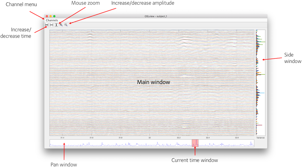
OSLview displays a time window of data from all channels for a particular sensor type. You can choose the sensor type from the 'Channels' menu. From left to right, the buttons on the top of the window are

Summary Statistics

In addition to displaying the data in the main window, OSLview also displays summary statistics of the data in the Pan Window and Side Window. The Side Window shows the variance of each channel over all time points (right clicking this window brings up a context menu that allows this to be changed to kurtosis). The Pan Window shows the variance over all channels at each time point.

Note that for more details on oslview, see:

https://ohba-analysis.github.io/osl-docs/matlab/osl_example_oslview.html

The unpreprocessed data here is very messy, with many artefacts, low frequency noise and line noise (50Hz plus its harmonics). We will now do some temporal filtering to help start removing these. First, close oslview.

FILTERING: BAND-PASS AND NOTCH FILTERING

Some artefacts are relatively easy to remove by filtering. Line noise is often filtered out by using an appropriate notch filter. Also, low frequency drifts and high frequency noise can be removed by filtering. This is what we will do next.

We have already set the SPM file names for the input into the filtering above, but if we needed to setup them up here, we would use something like:

spm_files=[];
for subnum = 1:length(spm_files_basenames) % iterates over subjects
    spm_files{subnum}=fullfile(workingdir,spm_files_basenames{subnum});
end

We then pass these inputs to the SPM function osl_filter to band pass filter between 0.1Hz and 120Hz. As well as removing noise outside this frequency range, this reflects the fact that we have decided that we do not need to keep any signal that may be outside this frequency range in our planned event related field (ERF) analysis.

The resulting filtered data set will get the prefix 'f' preceding the file name.

for subnum = 1:length(spm_files) % iterates over subjects
    D=spm_eeg_load(spm_files{subnum});
    D=osl_filter(D,[0.1 120],'prefix','f');
end

In a second step we reduce the line noise around 50 Hz, and around 100Hz (the first harmonic of the line noise). Please remember that filtering is blind to the origin of your signal, it might remove both line noise and any other neural signals at the same frequency, for example real gamma activity. However, for our practical and the goal of looking at event-related fields (ERFs) this approach is sufficient. As a general rule, always double-check your data after filtering to avoid bad surprises later in the processing pipeline - e.g. you can do this using oslview.

for subnum = 1:length(spm_files_basenames) % iterates over subjects
    spm_files{subnum}=fullfile(workingdir, ['f' spm_files_basenames{subnum}]);
end

for subnum = 1:length(spm_files) % iterates over subjects
    D=spm_eeg_load(spm_files{subnum});
    D=osl_filter(D,-[48 52],'prefix',''); % removes line noise using a notch filter
    D=osl_filter(D,-[98 102],'prefix','f'); % removes harmonic of line noise using a notch filter
end

DOWNSAMPLING

The data we are working with here has already been downsampled to 250 Hz when the Maxfilter was run on it. But we will now do further downsampling to 150Hz as this helps to speed things up even more, and we do not need information at high frequency in this particular analysis.

[Note that doing downsampling here is particularly necessary if movement compensation has been used when running Maxfilter, as this stops you from doing downsampling as part of the Maxfilter call.]

Also, as a rule of thumb, always filter first (especially low-pass), before downsampling to avoid any aliasing issues (https://en.wikipedia.org/wiki/Nyquist_frequency#Aliasing).

We first set the filenames used in following steps. Since we did both a highpass and a stopband (aka notch) filter, the prefix here needs to be 'ff'.

clear spm_files;
for subnum = 1:length(spm_files_basenames) % iterates over subjects
    spm_files{subnum}=fullfile(workingdir, ['ff' spm_files_basenames{subnum}]);
end

We now do the downsampling. Regarding the output, by default, the downsampled data set will get the prefix 'd' (preceding any other prefixes acquired before). This does the downsampling:

S=[];
for subnum=1:length(spm_files) % iterates over subjects
    S.D=spm_files{subnum};
    S.fsample_new = 150; % in Hz
    D = spm_eeg_downsample (S);
end

LOAD THE DOWNSAMPLED SPM M/EEG OBJECT

First, we need to set the filenames to correspond to the SPM MEEG object at the current point in the analysis. Hence, we need to use the prefixes 'dff' (2x filtered and then downsampled):

clear spm_files;
for subnum = 1:length(spm_files_basenames) % iterates over subjects
    spm_files{subnum}=fullfile(workingdir,['dff' spm_files_basenames{subnum}]);
end

We then will load in the SPM M/EEG object:

subnum = 1;
D = spm_eeg_load(spm_files{subnum});

Let's have a look at the SPM object. Note that it is continuous data, with 139200 time points at 150Hz. We will epoch the data later.

D

Let's have a look at the continuous data using oslview, now that it has been temporally filtered and downsampled. You'll see that while there is a big improvement, there are still exceptionally big artefacts in this data, especially at the end of the scan. This severity of artefact is not normal for good quality MEG and EEG data, but it serves well for demonstrating the power of good preprocessing.

Close oslview.

oslview(D);

AUTOMATED BAD SEGMENT/CHANNEL DETECTION

As we have seen, even after temporal filtering there can be large artefacts left in the data. Hence, we next perform bad segment/channel detection. This can be done either manually or automatically.

We will first do this automatically using the function osl_detect_artefacts.

Note that in the code below we first create a copy of the D objects using spm_eeg_copy. These will be the new SPM MEEG objects that will eventually have the bad segments/channels indicated in them. Here we represent bad segment/channel detection in the filename using the prefix 'B'

The MEEG object will be saved by the D.save (containing the marked bad segments/channels).

clear spm_files;
for subnum = 1:length(spm_files_basenames) % iterates over subjects
    spm_files{subnum}=fullfile(workingdir,['dff' spm_files_basenames{subnum}]);

    S=[];
    S.D=spm_files{subnum};
    S.outfile=prefix(spm_files{subnum},'B');
    D=spm_eeg_copy(S); % copy D object and add B prefix

    modalities = {'MEGMAG','MEGPLANAR'};

    % look for bad channels
    D = osl_detect_artefacts(D,'badchannels',true,'badtimes',false,'modalities',modalities);

    % then look for bad segments
    D = osl_detect_artefacts(D,'badchannels',false,'badtimes',true,'modalities',modalities);

    D.save;
end

Note that the bad segments/channels are not actually removed from the data, they are instead marked as bad, so that they can be optionally excluded from future parts of the analysis.

We now view the automatically marked segments/channels using oslview.

D=oslview(D);

The start of any bad segments are indicated with a dashed green line, and the end with a dashed red line.

Bad channels have their data plotted as dashed lines.

There are a lot of artefacts now marked in this data!

See https://ohba-analysis.github.io/osl-docs/matlab/osl_example_preprocessing_detect_artefacts.html for more info on this automated approach, including how to select data that exludes bad channels/segments. Close oslview.

MANUAL BAD SEGMENT/CHANNEL DETECTION USING OSLVIEW

There is also the option to run manual bad segment/channel detection using oslview itself. We can do this as an alternative, or in addition, to the automated bad segment/channel detection described above.

Here we now run the manual dection on the data without the automated bad segment/channel detection having been done (i.e. using the data with the 'dff' prefix as input).

clear spm_files;
for subnum = 1:length(spm_files_basenames) % iterates over subjects
    spm_files{subnum}=fullfile(workingdir,['dff' spm_files_basenames{subnum}]);

    S=[];
    S.D=spm_files{subnum};
    S.outfile=prefix(spm_files{subnum},'B');
    D=spm_eeg_copy(S); % copy D object and add B prefix

    D=oslview(D);
    D.save();
end

This data has some exceptionally bad artefacts in. Mark the segments at around 325s, 380s and 600s as bad, as well as everything from 650 seconds to the end. Marking is done by right-clicking in the proximity of the event and click on 'Mark Event'. A first click (green dashed label) marks the begin of a bad period, another second click indicates the end (in red). This will mean that we are not using about half of the data. But with such bad artefacts this is the best we can do. We can still obtain good results with what remains.

Don't forget to repeat this in both MEGPLANAR and MEGMAG modalities! You can switch between modalities using the Channels drop down menu at the top of the oslview window.

The MEEG object will be saved by the D.save call (containing the marked bad segments).

As with the automated approach, the bad segments are not actually removed from the data, they are instead marked as bad, so that they can be optionally excluded from future parts of the analysis.

Note that if you had multiple subjects/sessions, this process would need to be repeated for each one.

MANUAL AFRICA DENOISING

In a next step we will run AFRICA denoising. AFRICA uses independent component analysis (ICA) to decompose sensor data into a set of maximally independent time courses. Using this framework, sources of interference such as eye-blinks, ECG artefacts and mains noise can be identified and removed from the data or at least attenuated. In this practical we will use manual artefact rejection by looking at the time courses and sensor topographies of each component and rejecting those that correlate with EOG and ECG measurements. The user interface displays the time course, power spectrum and sensor topography for each component. These components are sorted based on one of a number of metrics, which you can toggle using the dropdown menu. For more information about AFRICA and how to use it, please see the AFRICA wiki manual on

https://ohba-analysis.github.io/osl-docs/pages/docs/preprocessing.html#africa

We first set the SPM M/EEG object filenames for the data to be input into AFRICA:

clear spm_files;
for subnum = 1:length(spm_files_basenames) % iterates over subjects
    spm_files{subnum}=fullfile(workingdir,['Bdff' spm_files_basenames{subnum}]);
end

We next create a copy of the D object using spm_eeg_copy. This will be the new SPM MEEG object that will eventually have AFRICA denoising in it. Note that here we will represent AFRICA denoising in the filename using the prefix 'A':

subnum = 1;
S=[];
S.D=D;
S.outfile=prefix(spm_files{subnum},'A');
D=spm_eeg_copy(S);

We will now run AFRICA. Once the ICA is computed, a window should be display. You can scroll through components by clicking on the sub-plot on the right (which shows the components ordered by the specified criteria), and then using the up/down cursor keys.

We will now identify the two components that correlate with the EOG and ECG measurements and mark them for rejection using the red cross.

D = osl_africa(D,'used_maxfilter',1,'do_ident','manual'); % Make sure you specify you want to do manual rather than automatic rejection
D.save(); % You need to save the MEEG object to commit marked bad components to disk

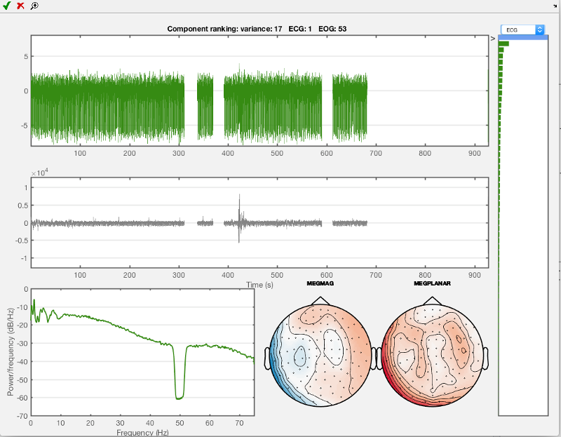
Use the drop-down menu to go to ECG (electrocardiogram, heartbeat-related electrical activity). Shown below is the first component that you should see then. This is the component that is most correlated to the ECG channel measurements. Mark this first component which should look like the one below for rejection using the red cross.

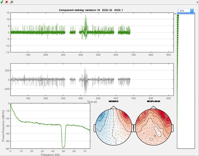
Now do the same for the eye movement component, use 'EOG' in the drop-down menu and the first component you see should look like the one shown below. Mark this one for rejection as well. Then close the AFRICA window to save the changes.

Just close the window when finished to save your results.

Note that if you had multiple subjects/sessions, this process would need to be repeated for each one.

VISUALISING AFRICA DENOISED CONTINUOUS DATA

After having done AFRICA denoising, let's have a look at the effect this has on our data quality. AFRICA has saved an 'online montage' attached to the current D object, which you should see indicate when you look at the D object:

D

These online montages are linear combinations of the original sensor data that can be used to basically represent any linear operation. This can be very convenient since it avoids amassing data without need. Here, for example, our first online montage has been generated by AFRICA and represents the data after having removed both the most important ECG and EOG components.

You can use the has_montage function to list the available montages

has_montage(D)

Now we can switch to any montage we want. D_pre_africa switches to the original, raw data while D_africe switches to the AFRICA denoised data. Have a look at the output to see the difference.

D_pre_africa=D.montage('switch',0)

D_africa=D.montage('switch',1)

Keep in mind that just switching ( as in typing D.montage('switch',0) ) is not enough, you need to assign the switched montage to a variable. It will switch, but there will be no new object with the online montage applied. So always use it in the way shown above. Examine the content of each object by just typing D_pre_africa and D_africa.

Now we plot some data to have a look at the differences between raw and denoised data.

figure;
subplot(2,1,1);
plot(D_pre_africa.time(1:10000),D_pre_africa(308,1:10000)); % takes first 10000 sample points
title('ECG channel')
xlim([10 20]);
xlabel('Time (s)');

subplot(2,1,2);
plot(D_pre_africa.time(1:10000),D_pre_africa(306,1:10000)); % takes first 10000 sample points
title('ECG contaminated channel')
xlim([10 20]);
hold on;
plot(D_africa.time(1:10000),D_africa(306,1:10000),'r');
xlim([10 20]);
xlabel('Time (s)');
legend({'pre AFRICA' 'post AFRICA'});

You should see something like this:

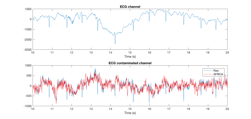
The first part of this figure plots the ECG channel included in the recording as reference (channel 308). In the second part we plot the two different variants of the same data set, the first shows the raw time series, and the second shows AFRICA run on it and cleaned (EOG / ECG attenuated). You can see that there is some commonalities between the ECG and some part of the raw, uncleaned time-series in the data (at least in that channel, 306), but that this is gone in the AFRICA denoised version. That means that AFRICA has removed most of the ECG contaminated parts in the signal. This is clearly superior to filtering, for example you should see one bump that looks a bit like a heart beat component, but it is not in the ECG channel. After AFRICA denoising this downward deflection is still there, which is desirable, since it is not ECG. Filtering would just have removed all these bumps equally, including any neuronal signal in that frequency range.

EPOCHING OF DATA

Now we will epoch the data into trials.

Here the epochs are set to be from -1000ms to +2000ms relative to the triggers in the MEG data. We also specify the trigger values for each of the 4 epoch types of interest (motorcycle images, neutral faces, fearful faces, happy faces). The codes used on the trigger channel for this experiment were:

1  =  Neutral face
2  =  Happy face
3  =  Fearful face
4  =  Motorbike
11 =  Break between blocks
12 =  Green fixation cross (response trials)
13 =  Red fixation cross (following green on response trials)
14 =  Red fixation cross (non-response trials)
19 =  Midway break
33 =  Introduction screen

Note that we are only interested in the first 4 event codes listed here for today's workshop.

As before, here we set filenames used for the following step. Prefix is now 'ABdff'. The following code setups the trial definition and then finds the relevant events in the continuous data, storing the resulting trial structure in epochinfo

clear spm_files;
for subnum = 1:length(spm_files_basenames) % iterates over subjects
    spm_files{subnum}=fullfile(workingdir,['ABdff' spm_files_basenames{subnum}]);
end

clear epochinfo;
for i=1:length(spm_files) % Iterating over subjects

    % define the trials we want from the event information
    S2 = [];
    S2.D = spm_files{i};
    D_continuous=spm_eeg_load(spm_files{i});
    D_continuous=D_continuous.montage('switch',0);

    pretrig = -1000; % epoch start in ms
    posttrig = 2000; % epoch end in ms
    S2.timewin = [pretrig posttrig];

    % event definitions
    S2.trialdef(1).conditionlabel = 'Neutral face';
    S2.trialdef(1).eventtype = 'STI101_down';
    S2.trialdef(1).eventvalue = 1;
    S2.trialdef(2).conditionlabel = 'Happy face';
    S2.trialdef(2).eventtype = 'STI101_down';
    S2.trialdef(2).eventvalue = 2;
    S2.trialdef(3).conditionlabel = 'Fearful face';
    S2.trialdef(3).eventtype = 'STI101_down';
    S2.trialdef(3).eventvalue = 3;
    S2.trialdef(4).conditionlabel = 'Motorbike';
    S2.trialdef(4).eventtype = 'STI101_down';
    S2.trialdef(4).eventvalue = 4;

    S2.reviewtrials = 0;
    S2.save = 0;
    S2.epochinfo.padding = 0;
    S2.event = D_continuous.events;
    S2.fsample = D_continuous.fsample;
    S2.timeonset = D_continuous.timeonset;

    [epochinfo{i}.trl, epochinfo{i}.conditionlabels] = spm_eeg_definetrial(S2);
end

We can visualise the timings of the information in epochinfo. This shows the different trial types alongside the samples that have been marked as bad, in continuous time. The start of a trial is marked with an 'o', and the end is marked with an 'x'. Bad trials are shown in black.

subnum=1;
report.trial_timings(spm_files{subnum}, epochinfo{subnum});

The following code now actually uses the 360 trials defined in epochinfo to do the epoching using a call to osl_epoch. Note that any trials that overlapped at all with any bad segments in the continuous data, will be marked as bad in the epoched data.

for i=1:length(spm_files) % Iterating over subjects
    S3 = epochinfo{i};
    S3.D = spm_files{i};
    D = osl_epoch(S3);
end

After epoching, data will be stored in a file with the prefix 'e', preceding all the other prefixes acquired during preprocessing.

EXAMINING THE EPOCHED DATA

Now we'll take a look at our preprocessed data so far.

To load in the epoched data, we need to load in the file with prefix 'eABdff'.

clear spm_files;
for subnum = 1:length(spm_files_basenames) % iterates over subjects
    spm_files{subnum}=fullfile(workingdir,['eABdff' spm_files_basenames{subnum}]);
end

D = spm_eeg_load(spm_files{subnum});

Have a look at the SPM object. Note that this is now epoched data, with:

D

Display a list of trial types:

D.condlist

Display a condition labels for each trial:

D.conditions

Display time points (in seconds) per trial (i.e. the time within a trial):

D.time

Any trials that overlap with bad segments that we marked as bad on the continuous data, will now be marked as bad trials in the epoched data.

We can see this clearly if we use the function report.trial_timings to look at the epoched data in continuous space. Any trials that overlap with bad segments are now marked bad, and are shown in black.

report.trial_timings(D);

We can see the indices for bad trials using:

disp('Bad trial indices:');
disp(D.badtrials);

We can also see the indices for any bad channels.

disp('Bad channel indices:');
disp(D.badchannels);

We can also view summary plots of the bad trials. This produces separate figures for MEGPLANARS and MEGMAGS. These show the standard deviation of the data in each trial/epoch, and a histogram of the standard deviation of the data in each trial/epoch. These are shown with (top half), or without (bottom half), the bad trials. Trials marked as bad are shown as red astrices, and trials marked as good are green astrices. You may need to zoom in on the second (from the top) subplot to see the green, good trials.

report.bad_trials(D);

We can also view bad MEG channel information:

modalities = {'MEGMAG','MEGPLANAR'};
report.bad_channels(D, modalities);

We will now perform outlier/bad trial detection directly on the epoched data to refine the marking of bad trials further.

AUTOMATED BAD TRIAL/CHANNEL DETECTION

We can either perform manual or automated bad trial detection.

We will first do this automatically using the function osl_detect_artefacts. This can also find bad channels.

Note that in the code below we first create a copy of the D objects using spm_eeg_copy. This will be the new SPM MEEG objects that will eventually have the bad trials indicated in them. Here we represent bad epoch detection in the filename using the prefix 'R':

clear spm_files;
for subnum = 1:length(spm_files_basenames) % iterates over subjects
    spm_files{subnum}=fullfile(workingdir,['eABdff' spm_files_basenames{subnum}]);

    S=[];
    S.D=spm_files{subnum};
    S.outfile=prefix(spm_files{subnum},'R');
    D=spm_eeg_copy(S); % copy D object and add R prefix

    modalities = {'MEGMAG','MEGPLANAR'};
    % look for bad channels
    D = osl_detect_artefacts(D,'badchannels',true,'badtimes',false,'modalities',modalities);

    % then look for bad segments
    D = osl_detect_artefacts(D,'badchannels',false,'badtimes',true,'modalities',modalities);
    D.save;
end

Note that the bad trials/channels are not actually removed from the data, they are instead marked as bad, so that they can be optionally excluded from future parts of the analysis.

As before, we can now see the indices for any bad trials and channels. This will be a combination of those trials that overlapped with bad epochs on the continuous data, and trials that have just now been identified as bad using the automated bad trial detection on the epoched data.

disp('Bad trial indices:');
disp(D.badtrials);

disp('Bad trial indices:');
disp(D.badchannels);

Again, can also view summary plots of the bad trials

report.bad_trials(D);

And we can view the different trial types alongside the samples that have been marked as bad, in continuous time. The start of a trial is marked with an 'o', and the end is marked with an 'x'. Bad trials are shown in black.

report.trial_timings(D);

MANUAL BAD TRIAL/CHANNEL DETECTION

Generally, automated bad trial/channel detection is sufficient and is recommended. However, there is also the option to run manual bad trial/channel detection using a Fieldtrip interactive tool. We can do this as an alternative, or in addition, to the automated bad trial/channel detection done above.

Here we will run the manual dection on the data that has already had the automated bad trial/channel detection done (i.e. using the data with the 'ReABdff' prefix as input).

clear spm_files
for subnum = 1:length(spm_files_basenames) % iterates over subjects
    spm_files{subnum}=fullfile(workingdir,['ReABdff' spm_files_basenames{subnum}]);

    S=[];
    S.D=spm_files{subnum};
    S.outfile=prefix(spm_files{subnum},'R');
    D=spm_eeg_copy(S); % copy D object and add R prefix

    D=osl_rejectvisual(D,[-0.2 0.4]);
    D.save();
end

The first channel type that is loaded up is the 'EOG' channel, so you will need to pass over this - so just press the "quit" button. This will bring up the next figure which will show the magnetometers. You can choose the metric to display - it is best to stick to the default, which is variance. This metric is then displayed for the different trials (bottom left), the different channels (top right), and for the combination of the two (top left). You need to use this information to identify those trials and channels with high variance and remove them.

Again, we can visualise the bad trial information:

report.bad_trials(D);

EXAMINE AND VISUALISE EPOCHED DATA

The pre-processing is now completed.

We will finish by looking at the benefits of bad trial/segment/channel detection and AFRICA by computing a rudimentary event related field (ERF) for the motorbike trials

First, we set the new SPM M/EEG object filenames for epoched data to be used in visualisation of ERFs

spm_files=[];
for subnum = 1:length(spm_files_basenames) % iterates over subjects
    spm_files{subnum}=fullfile(workingdir,['RReABdff' spm_files_basenames{subnum}]);
end

Next, we load in the data:

subnum = 1;
D = spm_eeg_load(spm_files{subnum});

We want to look at data without any of the effects AFRICA of clean up. to get this, we make sure the montage is set to 0 (i.e. no montage, corresponding to the raw sensors):

D=D.montage('switch',0)

We can now identify motorbike trials using the indtrial function. E.g.:

motorbike_trls = indtrial(D,'Motorbike');

This gives all trials for the motorbike condition in the data (regardless of whether they contain good or bad data segments).

We then identify channels of certain types using the indchantypes function. E.g. identify the channel indices for the planar gradiometers and for the magnetometers (what you have available may depend on the actual MEG device). Note that you can use 'MEGMAG' to get the magnetometers, and D.chantype gives you a list of all channel types by index.

planars = D.indchantype('MEGPLANAR');
magnetos = D.indchantype('MEGMAG');

These correspond to all channels of those types in the data (regardless of whether they are good or bad channels).

We can then access the actual epoched MEG data using the syntax: D(channels, samples, trials). E.g. here we will plot a figure showing all the trials for the motorbike condition in the 135th MEGPLANAR channel. Note that the squeeze function is needed to remove single dimensions for passing to the plot function, and D.time is used to return the time points relative to the trigger events (t=0 is time of stimulus onset) in seconds.

figure('units','normalized','outerposition',[0 0 0.5 0.4]);
subplot(1,2,1); % this plots all single trials
plot(D.time,squeeze(D(planars(135),:,motorbike_trls)));
xlabel('Time (seconds)','FontSize',15);
ylabel('Magnetic field gradient (fT/mm)','FontSize',15);
set(gca,'FontSize',15)
title('Raw event-related field, single trials','FontSize',15)

subplot(1,2,2);
plot(D.time,squeeze(mean(D(planars(135),:,motorbike_trls),3))); % this averages over trials
xlabel('Time (seconds)');
ylabel('Magnetic field gradient (fT/mm)','FontSize',15);
set(gca,'FontSize',15)
title('Raw event-related field, average','FontSize',15)

You should see something like this:

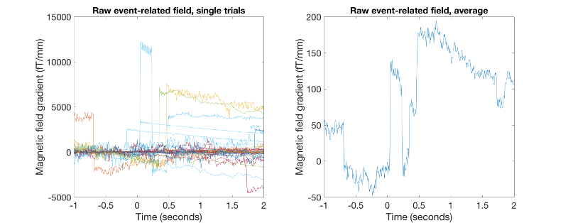
As you will notice, the ERF, both single trials and the average obtained are actually not usable at all. However, we should bear in mind that this data is averaging over all data including trials that we have marked as bad.

We will now look at the cleaned ERFs by only using good trials and channels, and seeing the effects of using AFRICA

First, we identify the good motorbike image trials. Note that indtrial includes good AND bad trials, so bad trials need to be excluded. 'good' finds the trials that are not bad.

good_motorbike_trls = D.indtrial('Motorbike','good');

To see the effects of AFRICA, we will make use of the online montages. Note that the online montage got carried over when doing the epoching. So there is no need to do epoching on both the 'raw' and AFRICA denoised data separately. Epoching on the raw data containing the AFRICA montage allows you to switch between raw and AFRICA denoised data after epoching without problems. So we can use online montage 1 ('AFRICA denoised data'). Again, keep in mind to assign it a new object (e.g. D_africa):

D_africa=D.montage('switch',1)

% Whereas our pre-AFRICA data corresponds to:

D_pre_africa=D.montage('switch',0)

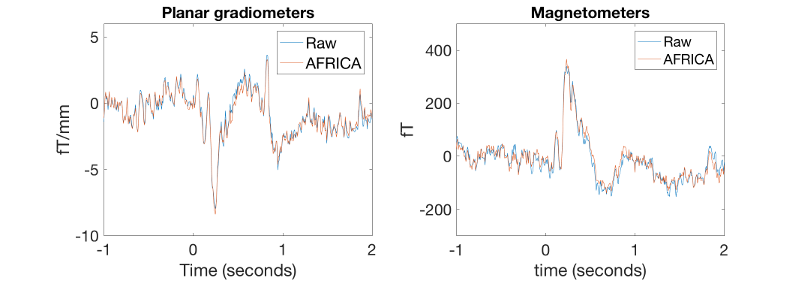
Now let us plot a cleaned rudimentary ERF for both the pre-AFRICA and post-AFRICA denoised data, but after having excluded the bad segments/channels and the bad trials from the artifact rejection. Now, the ERFs should look much better. Also, let us see how much the task-related activity, i.e. the ERF differs between 'raw' and AFRICA denoised data.

This should give you some nice event-related fields.

figure('units','normalized','outerposition',[0 0 0.4 0.3]);
subplot(1,2,1); % plots gradiometers, raw
plot(D_pre_africa.time,squeeze(mean(D_pre_africa(planars(135),:,good_motorbike_trls),3)));
xlabel('Time (seconds)','FontSize',15);ylim([-10 6])
set(gca,'FontSize',15)
ylabel(D_pre_africa.units(planars(1)),'FontSize',15);

hold on;
subplot(1,2,1); % plots gradiometers, AFRICA denoised
plot(D_pre_africa.time,squeeze(mean(D_africa(planars(135),:,good_motorbike_trls),3)));
xlabel('Time (seconds)','FontSize',15);ylim([-10 6])
legend({'Raw' 'AFRICA'},'FontSize',15);
set(gca,'FontSize',15)
title('Planar gradiometers','FontSize',15)

subplot(1,2,2); % plots magnetometers, raw
plot(D_pre_africa.time,squeeze(mean(D_pre_africa(magnetos(49),:,good_motorbike_trls),3)));
xlabel('time (seconds)','FontSize',15);ylim([-300 500])
ylabel(D_pre_africa.units(magnetos(1)),'FontSize',15);
set(gca,'FontSize',15)

hold on;
subplot(1,2,2); % plots magnetometers, AFRICA denoised version
plot(D_africa.time,squeeze(mean(D_africa(magnetos(49),:,good_motorbike_trls),3)));
xlabel('time (seconds)');ylim([-300 500])
ylabel(D_africa.units(magnetos(1)),'FontSize',15);
set(gca,'FontSize',15)
legend({'Raw' 'AFRICA'})
title('Magnetometers','FontSize',15)

These ERFs now should look much better than before. They should look like this:

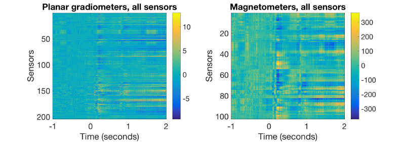
Now we will plot a 2D image of all cleaned ERFs across all sensors (204 planar gradiometers and 102 magnetometers):

figure('units','normalized','outerposition',[0 0 0.4 0.3]); % plots gradiometers
subplot(1,2,1);imagesc(D_africa.time,[],squeeze(mean(D_africa([planars(:)],:,good_motorbike_trls),3)));
xlabel('Time (seconds)','FontSize',20);
ylabel('Sensors','FontSize',15);colorbar
title('Planar gradiometers, all sensors','FontSize',15)
set(gca,'FontSize',15)

subplot(1,2,2); % plots magnetometers
imagesc(D_africa.time,[],squeeze(mean(D_africa([magnetos(:)],:,good_motorbike_trls),3)));
xlabel('Time (seconds)','FontSize',15);
ylabel('Sensors','FontSize',15);colorbar
title('Magnetometers, all sensors','FontSize',15)
set(gca,'FontSize',15)

These 2D images should correspond to the curves before. They should look like this:

PLOTTING EVENT-RELATED TOPOGRAPHIES AT DEFINED LATENCIES

To plot a cleaned rudimentary ERF topography (here at a relatively late latency) over all good trials for the pre-AFRICA data, do:

figure('units','normalized','outerposition',[0 0 0.4 0.4],'name','Without AFRICA denoising');
topo=squeeze(mean(D_pre_africa(:,188,good_motorbike_trls),3));
sensors_topoplot(D_pre_africa,topo,{'MEGPLANAR' 'MEGMAG'},1);

The obtained topographies should correspond to the ERF time series at this time:

D_pre_africa.time(188)

They should look like this:

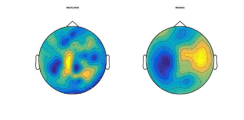
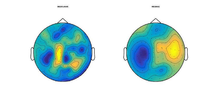
Now we do the same procedures for the AFRICA denoised online montage:

figure('units','normalized','outerposition',[0 0 0.4 0.4],'name','With AFRICA denoising');
topo2=squeeze(mean(D_africa(:,188,good_motorbike_trls),3));
sensors_topoplot(D_africa,topo2,{'MEGPLANAR' 'MEGMAG'},1);

They should look like this. Have a look at how different these topographies look. Here, AFRICA is not making a huge amount of difference to the ERFs and topographies; however, that is not always the case

EXERCISES

If you want to play around with the data and the cleaning approaches presented here, have a look at what happens when you remove more independent components during AFRICA. Also you can have a look at the interaction of oslview and AFRICA. For example, if you do not cut out the bad segments during oslview rejection, can you still get decent ERFs in the end? How many independent components would you need to remove to get some ERFs and are they still comparable to the ones generated earlier? Also, keep in mind that the data used here was meant to demonstrate the effect of artefacts in the data. Have a look at the other data sets presented during the following practical and see whether you can get similar success with even cleaner data, following the pipeline demonstrate in this practical here.

Published with MATLAB® R2018a