OSL Course Decoding Practical

In this practical, we will load some MEG data comprising presentation of words and images - for example, presentation of the word 'house' and presentation of an image of a house. As the two stimulus types have the same semantic meaning but very different visual features, we can investigate the temporal stages at which these different features are processed in the brain, and whether they converge on a similar representation after some higher level processing.

We will proceed through the following steps:

Contents

Section 1: Load single subject data

Much of the below analysis relies on training multivariate classifiers through cross validation. This approach can be quite time-consuming when applied to large datasets.

To save time, this practical will focus on the analysis of only a single subject's data. Nonetheless, group level data will be loaded at the last step to see how this result generalises to the group.

Let's clear up the workspace before beginning:

clc; clear all;close all;

Amend the following to be your OSL directory

OSLdir = '/Users/chiggins/Documents/MATLAB/osl/';

We will now load in the data

dir = [OSLdir '/osl-core/examples/OSL_decoding_data/'];
load([dir,'OSLDecodingPracticalData.mat']);
cd(dir)

About this data - for each condition (ie words and images), we now have brain data X and labels Y. These are in the same setup across modalities, with rows representing successive timepoints over trials, and columns representing different data dimensions.

Looking at our stimulus, Y_images has 8 columns, corresponding to the same 8 columns in Y_words. Each column denotes one of the stimuli, and is a 1 if that stimulus is presented at that timepoint and a 0 otherwise. So, for example, looking at Y_words, the first rows indicate that the word for stimulus 3 was presented; similarly, Y_images indicates that the first image presented was also stimulus 3 (the image presented always matched the word just shown, so Y_images and Y_words match throughout). The 8 stimuli used in the experiment were the following:

The neural data X_words and X_images is organised such that the rows correspond to the same timepoint and trial as the associated labels in Y_words and Y_images. Originally each column was an individual MEG sensor, with the following preprocessing applied:

We have taken an additional step of reducing the data dimensionality with PCA, so the columns of X now represent the first 50 principal components of the data.

Finally, although our rows represent time, the recording is not continuous in time throughout - we instead have a series of short trial epochs concatenated one after the other. The variable T_images and T_words indicate the number of samples in each trial, and so can be used to determine where each trial begins and ends.

Let's now identify some basic features:

ttrial = length(trial_timepoints)

ttrial =

    41

This is the number of datapoints in each trial. At a sampling rate of 100 samples/sec, this corresponds to samples taken from 0:400 msec following stimulus presentation.

Ntr = length(T_words)

Ntr =

   128

This is the number of independent trials (same number for words and images).

Ntr*ttrial
sum(T_images)
size(Y_images,1)
size(X_images,1)

ans =

        5248


ans =

        5248


ans =

        5248


ans =

        5248

The rows of our matrices represent timepoints, stacked over subsequent trials. T_images and T_words demarcate the number of timepoints in each trial, identifying where each trial begins and ends. As a sanity check, the total number of trials times timpoints should equal the sum of this T vector; which should also be the dimension of rows in our data X and design matrix Y.

p = size(X_words,2)

p =

    50

This is the data dimensionality - note this data has already been preprocessed, and the dimensionality has been reduced by principal component analysis - keeping only the first 50 principal components.

q = size(Y_words,2)

q =

     8

This is the stimulus dimensionality. We have 8 different stimuli. Let us now conduct a few sanity checks before proceeding:

unique(Y_words(:))

ans =

     0
     1

Note that all values of the stimulus Y are in a binary labelled format - that is, each column is either 1 or 0, denoting respectively whether that stimulus is on or off at that particular timepoint.

num_active_stimuli = sum(Y_words,2);
unique(num_active_stimuli)

ans =

     1

This tells us how many stimuli can be active at any point in time over the entire dataset. This tells us that our stimuli here are mutually exclusive; At every timepoint sampled, exactly one stimulus was active - no more, no less.

This is a very important point as far as methods are concerned. Decoding, the title of this practical, encompasses prediction of classes (ie classification) as well as prediction of continuous stimuli. While the approaches are extremely similar, the models used can be quite different. In particular, some of the methods discussed below (Logistic Regression, Linear Discriminant Analysis and Support Vector Machines) are only suitable for classification tasks - wherever the stimulus is continuous you can use a Gaussian model.

In the HMM-MAR toolbox, classification is handled by the following methods:

Whereas prediction of continuous stimuli is handled by the following:

Where our acronyms TUDA and TUCA stand for Temporally Unconstrained DECODING / CLASSIFICATION Analysis, respectively.

One remaining point is that our data should ideally be balanced over trials, to avoid introduction of biases into our classifiers. We can check this here:

nTrPerStim = sum(Y_images)./ttrial

nTrPerStim =

    16    16    16    16    16    16    16    16

Section 2: Setup Cross Validation Folds

Decoding analyses normally gauge their performance by testing how well a classifier generalises to unseen data. This motivates the process of cross validation, whereby we complete the following:

1. Isolate a subset of data for testing (the 'test set')

2. Train our classifiers on all the remaining data (the 'training set')

3. Apply the classifiers to the held-out test data and record their accuracy

4. Iterate through the above steps repeatedly until every trial has been in the test set once.

By default, the functions standard_classification(), standard_decoding(), tucacv() and tudacv() will automatically separate your data into training and test folds - here however, we will work through this manually to identify certain issues.

First, let us determine how many folds to use. If we wanted to maximise the amount of data each classifier is trained on, we would use as many training folds as we have trials of each stimulus:

NCV_optimal = min(nTrPerStim)

NCV_optimal =

    16

This is 'hold one out' cross validation. It uses the most data possible when training each classifier. It does, however, require quite long processing times - just to speed things up, let's work with 4 fold cross validation, where each test set contains a quarter of the total number of trials:

NCV = 4;

Y_per_trial = Y_images(1:ttrial:end,:);
[grouplabels,~] = find(Y_per_trial');
rng(1);
crossvalpartitions = cvpartition(grouplabels,'KFold',NCV);

The above code has called MATLAB's standard cvpartition function to break the available trials into multiple training and test partitions.

Note the information displayed in crossvalpartitions. We have 128 trials in total (each of length 41 timepoints). With 4 fold cross vaildation, these 128 trials are split into 4 different partitions, each containing a subset of 96 trials, which will be used as a training set (i.e. to learn a mapping between data and trial types); and 32 trials, which will be used to test how accurate the mapping is that has been learnt on the training set. The overall accuracy of the approach is then calculated by combining the results across the 4 test sets.

Note that using such a low number of cross validation folds speeds things up for the purposes of this practical. However, this has some unwanted side effects that make it undesirable in practice - namely it becomes much harder to ensure training sets are balanced, and you have fewer samples from which to train your classifiers.

Section 3: Training classifiers

Now, let's start training classifiers. There is a bewildering array of different classifiers that can be used, but for M/EEG data there is something of a consensus that linear classifiers perform sufficiently well in most scenarios. We will only work with linear classifiers here - this toolbox supports three different classifier types as follows:

We need only test one of these, but if you like you can try different options - we have found that results will vary slightly over different classifiers but not in particularly meaningful ways.

The standard_classification() function takes an approach that is mass univariate in time; that is, an independent classifier is trained for each timestep within the trials, giving us accuracy defined as a function of time. This can be thought of as a "sliding-window" approach, and critically assumes that there is a common timing (or synchronicity) in the response between trials. Later in the practical we will see how we can use an HMM-based approach to relax this assumption and do temporally unconstrained decoding/encoding.

options=[];
options.classifier='logistic';

We also want to specify the cross validation folds learned above:

options.c=crossvalpartitions;

So - let's now train a classifier over the presentation of words by passing the required sensor space MEG data, and trial labels to the function standard_classification. Note this will take a minute or two to run.

acc_words = standard_classification(X_words,Y_words,T_words,options);

CV iteration: 1 of 4
CV iteration: 2 of 4
CV iteration: 3 of 4
CV iteration: 4 of 4

And separately, let's also train a classifier over the presentation of images:

acc_images = standard_classification(X_images,Y_images,T_images,options);

CV iteration: 1 of 4
CV iteration: 2 of 4
CV iteration: 3 of 4
CV iteration: 4 of 4

Now let's plot the cross validated accuracy:

f1=figure('Position',[680 384 1084 714]);
plot(trial_timepoints,acc_images,'LineWidth',2);
hold on; plot(trial_timepoints,acc_words,'LineWidth',2);
set(gca,'fontsize',16);
set(gca,'LineWidth',2);
xlabel('Time (sec)','fontsize',16);
ylabel('Accuracy','fontsize',16);
title('Standard Decoding Accuracy');
chancelevel=0.125;
plot([trial_timepoints(1),trial_timepoints(end)],[chancelevel,chancelevel],'k--')
legend('Images','Words','Chance Level');

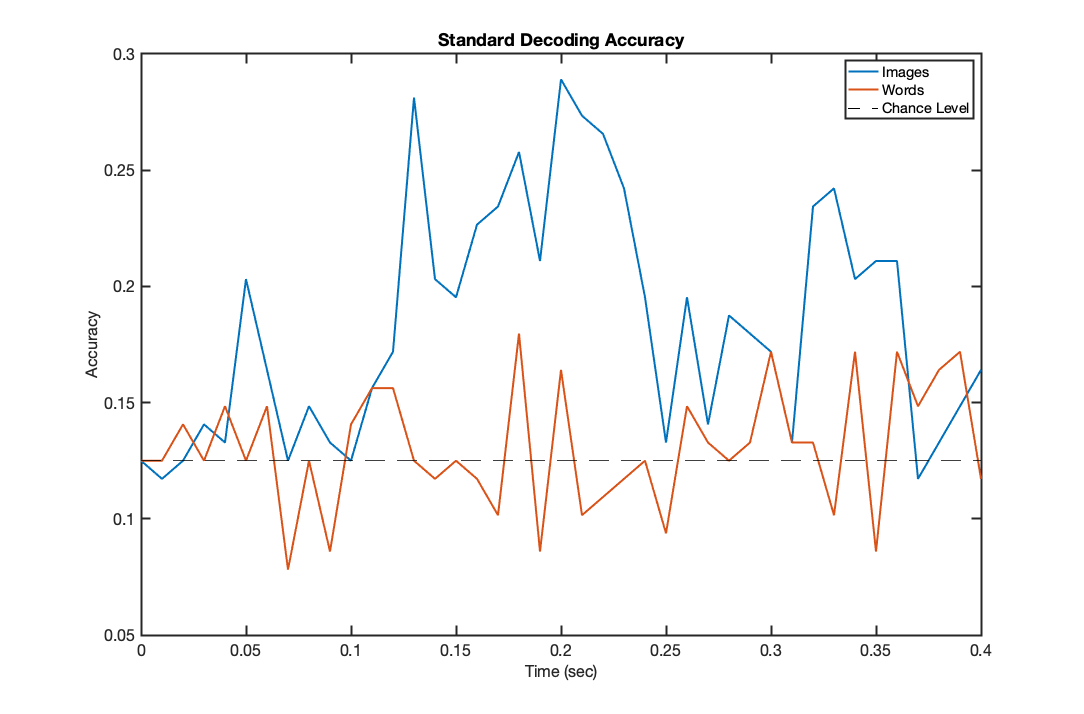
It is apparent that decoding of image data is significantly above chance, however decoding of word data is close to chance levels throughout. Is it statistically significantly above chance though? We can check this with a simple binomial test, selecting the time point of maximum accuracy

NCorrect = round(max(acc_words)*Ntr);
p_value = 1-binocdf(NCorrect,Ntr,chancelevel)

p_value =

    0.0272

This is the p value for the single best classification point - this will vary depending on the random allocation of cross validation folds and classifers used, but in most cases will be (only just) below 0.05. Noting that we have not corrected for multiple comparisons and have handpicked the single best point, this is not strong evidence for above chance decoding, but does suggest the result might be significant at the group level. Before we look at group level results though, let us analyse a different approach to decoding based on HMMs.

Section 4: train some HMM classifiers for comparison:

In the previous section, we trained classifiers independently on each timepoint. An alternative fully outlined in [Vidaurre et al, Cerebral Cortex, 2019] is to use a HMM model to infer a dynamic state sequence on each trial that best decodes the data. This has the advantage of grouping together timepoints that may be similarly distributed but poorly aligned over trials, and also accessing information content at a broader range of frequencies to decoders trained only on single timepoints. In other words, this relaxes the assumption that there is common timing (or synchronicity) in the response between trials, providing a temporally unconstrained decoding.

We will train a model now, using the same cross validation folds as before. For this model, we must enter a classifier type as before, with only the options of 'logistic' and 'LDA' now available.

options=[];
options.classifier='logistic';

These models infer a set of states that best describe the relationship between the data and the labels, states that can vary over trials to identify patterns that are poorly aligned. Unfortunately when conducting cross validation tests, this leaves no obvious way to infer each test trial's state timecourse (as these are normally determined by looking at the mapping between data and the labels, and for the testing we hold out the labels). We instead adopt a very conservative approach for each test trial, just using the average state timecourse fit over all trials in the training data, denoted here as CVmethod=1:

options.CVmethod=1;

We must also assign a number of states, denoted by the parameter K. More states means more decoding parameters, which will improve classification up to a point - however models with many states have much greater capacity to overfit to noise in the data, hence there is an optimal number of states that maximises the cross validated accuracy. We recommend starting with K=6 states:

options.K=6;

For direct comparison, we use the same cross validation folds as before:

options.c=crossvalpartitions;

So - let's now train a classifier over the presentation of words by passing the required sensor space MEG data, and trial labels to the function tucacv to do temporally unconstrained decoding. Note this will take a minute or two to run.

[~,acc_hmm_images,~,~] = tucacv(X_images,Y_images,T_images,options);
[~,acc_hmm_words,~,~] = tucacv(X_words,Y_words,T_words,options);

Model: 6 states, 4032 data samples, logistic regression model. 
Lapse: 1, order 1, offset 0 
MEX file was not used 
cycle 1 free energy = 23863.1 
cycle 2 free energy = 21290.2 
cycle 3 free energy = 20538.8,  relative change = -0.226039 
cycle 4 free energy = 20113.6,  relative change = -0.113409 
Model: 6 states, 4032 data samples, logistic regression model. 
Lapse: 1, order 1, offset 0 
MEX file was not used 

CV iteration: 1 of 4
Model: 6 states, 4032 data samples, logistic regression model. 
Lapse: 1, order 1, offset 0 
MEX file was not used 
cycle 1 free energy = 24074.7 
cycle 2 free energy = 21518.2 
cycle 3 free energy = 20779.9,  relative change = -0.224086 
cycle 4 free energy = 20348,  relative change = -0.115884 
Model: 6 states, 4032 data samples, logistic regression model. 
Lapse: 1, order 1, offset 0 
MEX file was not used 

CV iteration: 2 of 4
Model: 6 states, 4032 data samples, logistic regression model. 
Lapse: 1, order 1, offset 0 
MEX file was not used 
cycle 1 free energy = 23949.4 
cycle 2 free energy = 21359.6 
cycle 3 free energy = 20622,  relative change = -0.221677 
cycle 4 free energy = 20205.3,  relative change = -0.111287 
Model: 6 states, 4032 data samples, logistic regression model. 
Lapse: 1, order 1, offset 0 
MEX file was not used 

CV iteration: 3 of 4
Model: 6 states, 4032 data samples, logistic regression model. 
Lapse: 1, order 1, offset 0 
MEX file was not used 
cycle 1 free energy = 23878.8 
cycle 2 free energy = 21270.6 
cycle 3 free energy = 20546.4,  relative change = -0.217328 
cycle 4 free energy = 20140.5,  relative change = -0.108588 
Model: 6 states, 4032 data samples, logistic regression model. 
Lapse: 1, order 1, offset 0 
MEX file was not used 

CV iteration: 4 of 4
Model: 6 states, 4032 data samples, logistic regression model. 
Lapse: 1, order 1, offset 0 
MEX file was not used 
cycle 1 free energy = 25625.3 
cycle 2 free energy = 23128 
cycle 3 free energy = 22435.6,  relative change = -0.217044 
cycle 4 free energy = 22076.5,  relative change = -0.101205 
Model: 6 states, 4032 data samples, logistic regression model. 
Lapse: 1, order 1, offset 0 
MEX file was not used 

CV iteration: 1 of 4
Model: 6 states, 4032 data samples, logistic regression model. 
Lapse: 1, order 1, offset 0 
MEX file was not used 
cycle 1 free energy = 25665.8 
cycle 2 free energy = 23081.9 
cycle 3 free energy = 22388.4,  relative change = -0.211618 
cycle 4 free energy = 22032.9,  relative change = -0.0978472 
Model: 6 states, 4032 data samples, logistic regression model. 
Lapse: 1, order 1, offset 0 
MEX file was not used 

CV iteration: 2 of 4
Model: 6 states, 4032 data samples, logistic regression model. 
Lapse: 1, order 1, offset 0 
MEX file was not used 
cycle 1 free energy = 25752.5 
cycle 2 free energy = 23210.8 
cycle 3 free energy = 22509.8,  relative change = -0.216171 
cycle 4 free energy = 22143.6,  relative change = -0.101455 
Model: 6 states, 4032 data samples, logistic regression model. 
Lapse: 1, order 1, offset 0 
MEX file was not used 

CV iteration: 3 of 4
Model: 6 states, 4032 data samples, logistic regression model. 
Lapse: 1, order 1, offset 0 
MEX file was not used 
cycle 1 free energy = 25440.5 
cycle 2 free energy = 22835 
cycle 3 free energy = 22131.8,  relative change = -0.212552 
cycle 4 free energy = 21781.2,  relative change = -0.095815 
Model: 6 states, 4032 data samples, logistic regression model. 
Lapse: 1, order 1, offset 0 
MEX file was not used 

CV iteration: 4 of 4

Plotting the output:

f2=figure('Position',[680 384 1084 714]);
plot(trial_timepoints,acc_hmm_images,'LineWidth',2);
hold on; plot(trial_timepoints,acc_hmm_words,'LineWidth',2);
set(gca,'fontsize',16);
set(gca,'LineWidth',2);
xlabel('Time (sec)','fontsize',16);
ylabel('Accuracy','fontsize',16);
title('HMM decoding Accuracy')
chancelevel=0.125;
plot([trial_timepoints(1),trial_timepoints(end)],[chancelevel,chancelevel],'k--')
legend('Images','Words','Chance Level');

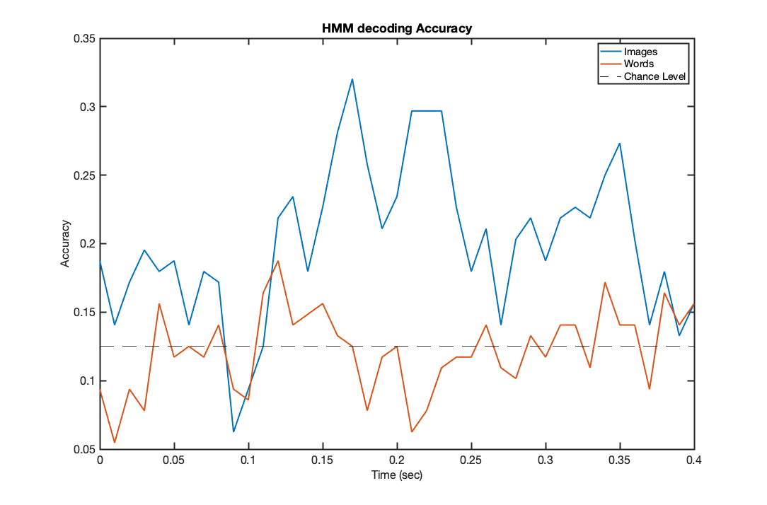
Computing the significance of the maximum accuracy point:

NCorrect = round(max(acc_hmm_words)*Ntr);
p_value = 1-binocdf(NCorrect,Ntr,chancelevel)

p_value =

    0.0153

For a direct comparison, let's plot the two classifers against each other:

f2=figure('Position',[680 384 1084 714]);subplot(1,2,1);
plot(trial_timepoints,acc_hmm_words,'LineWidth',2);
hold on; plot(trial_timepoints,acc_words,'LineWidth',2);
plot([trial_timepoints(1),trial_timepoints(end)],[chancelevel,chancelevel],'k--')
set(gca,'fontsize',16);
set(gca,'LineWidth',2);
xlabel('Time (sec)','fontsize',16);
ylabel('Accuracy','fontsize',16);
title('Decoding Words')
subplot(1,2,2);
plot(trial_timepoints,acc_hmm_images,'LineWidth',2);
hold on; plot(trial_timepoints,acc_images,'LineWidth',2);
plot([trial_timepoints(1),trial_timepoints(end)],[chancelevel,chancelevel],'k--')
set(gca,'fontsize',16);
set(gca,'LineWidth',2);
xlabel('Time (sec)','fontsize',16);
ylabel('Accuracy','fontsize',16);
legend('HMM','Standard')
title('Decoding Images')

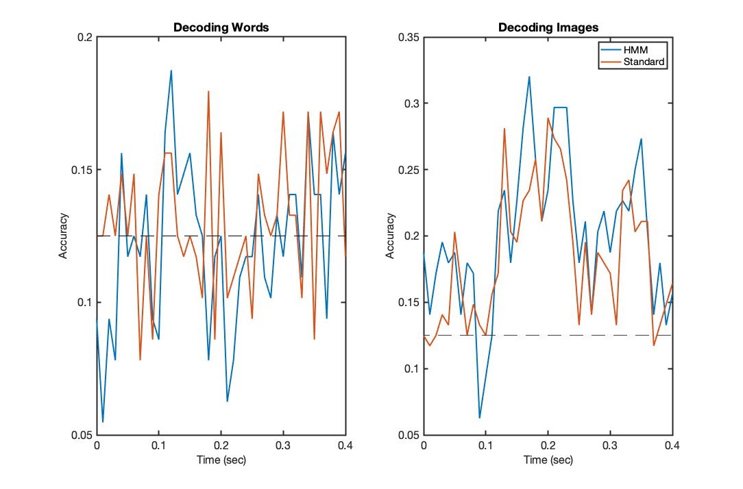
Again, these results will vary depending on the cross validation randomisation, but should show accuracy curves that are not wildly different. The performance on words data should be very similar, and only marginally above chance, if at all; whereas the performance on image data should show a very slight improvement in accuracy achieved by the HMM based models, that is probably most prominent in later timepoints where the representations may be more poorly aligned over trials.

Either way, any improvement in accuracy won't look groundbreaking, so what is the value of these HMM models? We argue the following three points:

1. The accuracy improvements shown here are conservative, as they are based on a mean state timecourse model. So the real HMM accuracy is probably much better.

2. When these are plotted at the group level, they more reliably outperform standard approaches, even with this conservative estimate

3. They additionally provide us with a key trial-specfic metric of when activity patterns are activated on different trials. So, they provide valuable information in between-trial temporal variability in stimulus processing

Section 5: Investigate temporal patterns of variation

One of the big advantages of the HMM classification framework is that it provides additional information regarding the timings of representations on an individual trial basis. This allows us to look at how the state timecourses on each trial relate to behaviour, such as reaction times.

Following presentation of images, participants were required to press a button. The timing of the button push was recorded as their reaction time - let's see if this correlates at all with the inferred timings of activity patterns on an individual trial basis.

Let's train an HMM model on image data, using the same parameters as above:

options=[];
options.K=6;
options.classifier='logistic';
options.verbose=false;
[tucamodel_images,Gamma_images] = tucatrain(X_images,Y_images,T_images,options);
Gamma_images_mean = squeeze(mean(reshape(Gamma_images,T_images(1),length(T_images),options.K),2));
T=T_images(1);

cycle 1 free energy = 29779.9 
cycle 2 free energy = 26579.6 
cycle 3 free energy = 25780.5,  relative change = -0.199792 
cycle 4 free energy = 25352,  relative change = -0.0967795 
Model: 6 states, 5376 data samples, logistic regression model. 
Lapse: 1, order 1, offset 0 
MEX file was not used 

Now Gamma_images denotes the inferred timings that different decoding models are activated. Let's first plot these to get a sense of the variation:

figure();
gammaRasterPlot(Gamma_images,T_images(1),[1:10:41],trial_timepoints([1:10:41]));
xlabel('Time (sec)','fontsize',16);
ylabel('Trial','fontsize',16);
title('Individual trial state timecourses');

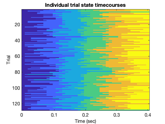
This should show quite a consistent structure of sequential states being activated, but some variation in the exact timings of when they are activated.

Do these times have any behavioural relevance? Let's determine their correlation with reaction times:

for k=1:options.K
    for t=1:T_images(1)
        [C(k,t),rho_pval(k,t)] = corr(Gamma_images(t:T_images(1):end,k),ReactionTimesImages);
    end
end

figure('Position',[680 602 931 496]);
subplot(2,1,1);
plot(trial_timepoints,Gamma_images_mean,'LineWidth',2);
set(gca,'fontsize',16);
xlabel('Time (sec)','fontsize',16);
ylabel('State probability','fontsize',16);
title('Mean State Timecourse')
subplot(2,1,2);
imagesc(C);colorbar('Position',[0.9234 0.1230 0.0229 0.3004]);
set(gca,'XTick',[1:10:41]);
set(gca,'XTickLabel',trial_timepoints([1:10:41]));
set(gca,'fontsize',16);
set(gca,'LineWidth',2);
xlabel('Time (sec)','fontsize',16);
ylabel('HMM state','fontsize',16);
title('Correlation with reaction times')

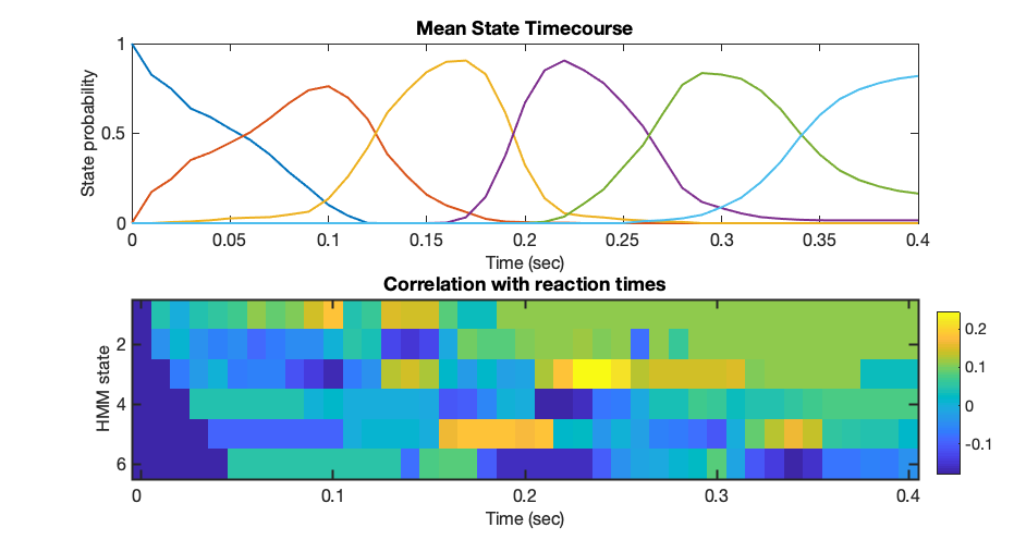
Once again, at the single subject level this is quite noisy, however you may notice a diagonal structure in the correlation pattern. If you compare the peak activation time of each state in the top graph with the correlation figure, you will find that trials where states are active ahead of the mean peak time correlate with lower (ie faster) reaction times; trials where states are active later than their mean peak correlate with longer (ie slower) reaction times.

This confirms that the inferred stages of processing are behaviourally relevant, and introduces another key variable into our analysis that allows us to quantify when things happen on individual trials. These correlate here with reaction times, but in other experiments with more cognitive components may be able to capture other meaningful differences in timing over trials that relate to higher order aspects of cognition.

Section 6: Classifier Generalisation tests

It appears our classifiers have learned something from the data. This is clear for the image classifiers, but somewhat ambiguous at the single subject level for word data. Let's now investigate what has been learned by testing how these classifiers generalise - by this, we mean to check whether classifiers trained on image data show any success decoding the equivalent word, and vice versa.

Let's now manually test this on word data. In order to do this, we need to understand briefly how these classifiers predict data. Logistic regression classifiers form their predictions by the following formula:

     |Y = logistic_sigmoid_transfer_function (X * beta)|

where beta are our regression coefficients. Note that in the code below the function tudabeta, given a precomputed TUDA model, returns these betas. The rest of the code predicts Y using these betas

On the other hand, if you are using LDA things are a bit different. LDA models fit a Gaussian distribution to the data of each class, and then determine the optimal classification boundary (the 'linear discriminant') between classes. This is done automatically below by the function LDApredict.

T=T_words(1);
if strcmp(options.classifier,'logistic')
    [~,Beta_coefficients] = tudabeta(tucamodel_images,Gamma_images_mean);
    Y_prediction=zeros(length(X_images),8);
    for t=1:T
        t_selected=[t:T:length(X_words)];
        Y_prediction(t_selected,:) = log_sigmoid(X_words(t_selected,:)*Beta_coefficients(:,:,t));
    end
    [~,hard_assignment_pred] = max(Y_prediction,[],2);
else %LDA
    Y_prediction = LDApredict(tucamodel_images,repmat(Gamma_images_mean,[length(T_images),1]),X_words);
    [~,hard_assignment_pred] = max(Y_prediction,[],2);
end
[~,hard_assignment_true] = max(Y_words,[],2);

Having found the highest probability prediction for each trial timepoint, contained in hard_assignment_pred, let us compare them to the ground truth, hard_assignment_true, to compute the accuracy:

accuracy = reshape(hard_assignment_pred==hard_assignment_true,T,length(T_words),1);
acc_time_imageOnWordData = mean(accuracy,2);

Now, let's do the same procedure, training a classifier on word data:

[tucamodel_words,Gamma_words] = tucatrain(X_words,Y_words,T_words,options);
Gamma_words_mean = squeeze(mean(reshape(Gamma_words,T_images(1),length(T_images),options.K),2));
T=T_images(1);

cycle 1 free energy = 32027.2 
cycle 2 free energy = 28870.1 
cycle 3 free energy = 28104.4,  relative change = -0.195184 
cycle 4 free energy = 27728.6,  relative change = -0.0874257 
Model: 6 states, 5376 data samples, logistic regression model. 
Lapse: 1, order 1, offset 0 
MEX file was not used 

And test its performance on the image data:

if strcmp(options.classifier,'logistic')
    [~,Beta_coefficients] = tudabeta(tucamodel_words,Gamma_words_mean);
    Y_prediction=zeros(length(X_images),8);
    for t=1:T
        t_selected=[t:T:length(X_images)];
        Y_prediction(t_selected,:) = X_images(t_selected,:)*Beta_coefficients(:,:,t);

    end
    [~,hard_assignment_pred] = min(abs(1-Y_prediction),[],2);
else %LDA
    predictions = LDApredict(tucamodel_words,repmat(Gamma_words_mean,[length(T_images),1]),X_images);
    [~,hard_assignment_pred] = max(predictions,[],2);
end
[~,hard_assignment_true] = max(Y_images,[],2);

Compute the overall accuracy:

accuracy = reshape(hard_assignment_pred==hard_assignment_true,T,length(T_images),1);
acc_time_wordOnImageData = mean(accuracy,2);

f1=figure('Position',[680 384 1084 714]);
plot(trial_timepoints,acc_time_imageOnWordData,'LineWidth',2);
hold on;plot(trial_timepoints,acc_time_wordOnImageData,'LineWidth',2);
chancelevel=0.125;
plot([trial_timepoints(1),trial_timepoints(end)],[chancelevel,chancelevel],'k--');
set(gca,'fontsize',16);
xlabel('Time (sec)','fontsize',16);
ylabel('Accuracy','fontsize',16);
title('Classifier Cross Generalisation');
legend({'Trained on images, tested on words','Trained on words, tested on images',...
    'Chance level'},'Location','EastOutside');

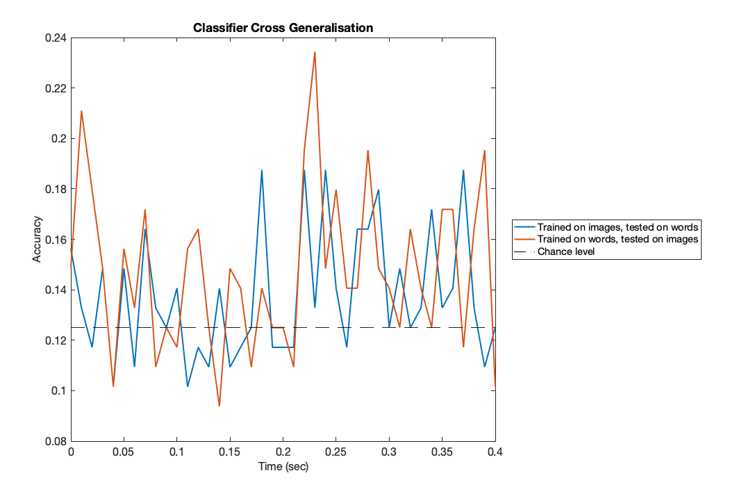
These results suggest an interesting trend - there may be above-chance decoding at later timepoints, reflecting some shared information between the representation of words and images appearing in MEG data approximately 300msec after initial presentation. But at the single subject level, these results are noisy and could easily be just due to chance. As a final step, let's load the group level results and analyse them.

Section 7: Group level analysis

The above analyses were conducted at the single subject level. At this level, some results were very clear (eg the decoding of images), while a number of others (eg decoding of words and cross-generalisation) displayed trends that may not have been significant. We will now load the group level results of the above generalisation tests, to see whether these results are significant at the group level.

The following results were obtained by running a 6 state HMM model using LDA classifiers and hold-one-out cross validation over all subjects. We will now load each subject's trial by trial accuracy:

load('OSLDecodingPracticalGroupLevelData.mat');

As decoding analyses are focussed on predictions of stimuli Y, for statistical analysis at the group level we can treat our results as just a series of concatenated predictions. Importantly, we are not concerned with comparing each individual's activity patterns for a stimulus (which can display little or no correlation over subjects) - all that matters is how well we could consistently predict stimuli as a function of time and the type of training data:

words = [];images = [];wordsOnImages = [];imagesOnWords = [];
for iSj=1:21
    words = cat(2,words,acc_hmm_words_sj{iSj});
    images = cat(2,images,acc_hmm_images_sj{iSj});
    wordsOnImages = cat(2,wordsOnImages,acc_hmm_wordsOnImageData_sj{iSj});
    imagesOnWords = cat(2,imagesOnWords,acc_hmm_imagesOnWordData_sj{iSj});
end

Find the mean accuracy over all trials:

word_groupacc = mean(words,2);
image_groupacc= mean(images,2);
wordOnImage_groupacc = mean(wordsOnImages,2);
imageOnWord_groupacc = mean(imagesOnWords,2);

and plot each of these:

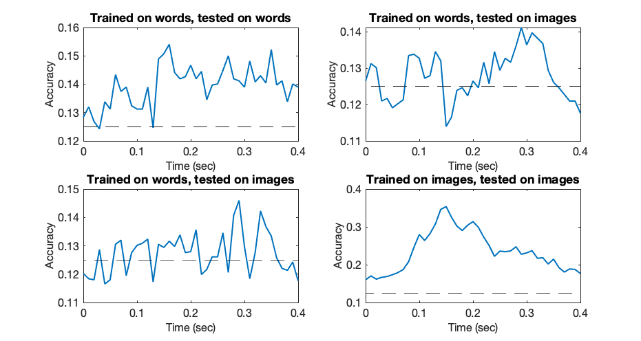
figure('Position',[680 602 931 496]);
subplot(2,2,1);
plot(trial_timepoints,word_groupacc,'LineWidth',2);
set(gca,'fontsize',16);
xlabel('Time (sec)','fontsize',16);
ylabel('Accuracy','fontsize',16);
title('Trained on words, tested on words');hold on;
plot([trial_timepoints(1),trial_timepoints(end)],[chancelevel,chancelevel],'k--')
subplot(2,2,2);
plot(trial_timepoints,imageOnWord_groupacc,'LineWidth',2);
set(gca,'fontsize',16);
xlabel('Time (sec)','fontsize',16);
ylabel('Accuracy','fontsize',16);
title('Trained on words, tested on images');hold on;
plot([trial_timepoints(1),trial_timepoints(end)],[chancelevel,chancelevel],'k--')
subplot(2,2,3);
plot(trial_timepoints,wordOnImage_groupacc,'LineWidth',2);
set(gca,'fontsize',16);
xlabel('Time (sec)','fontsize',16);
ylabel('Accuracy','fontsize',16);
title('Trained on words, tested on images');hold on;
plot([trial_timepoints(1),trial_timepoints(end)],[chancelevel,chancelevel],'k--')
subplot(2,2,4);
plot(trial_timepoints,image_groupacc,'LineWidth',2);
set(gca,'fontsize',16);
xlabel('Time (sec)','fontsize',16);
ylabel('Accuracy','fontsize',16);
title('Trained on images, tested on images');hold on;
plot([trial_timepoints(1),trial_timepoints(end)],[chancelevel,chancelevel],'k--')

Finally, let us quickly compute the significance of each peak accuracy point:

Ntr = size(words,2);
NCorrect = round(max(word_groupacc)*Ntr);
p_value_words = 1-binocdf(NCorrect,Ntr,chancelevel)
NCorrect = round(max(image_groupacc)*Ntr);
p_value_images = 1-binocdf(NCorrect,Ntr,chancelevel)
NCorrect = round(max(wordOnImage_groupacc)*Ntr);
p_value_wordsOnImages = 1-binocdf(NCorrect,Ntr,chancelevel)
NCorrect = round(max(imageOnWord_groupacc)*Ntr);
p_value_imageOnWords = 1-binocdf(NCorrect,Ntr,chancelevel)

p_value_words =

   3.7994e-06


p_value_images =

     0


p_value_wordsOnImages =

   5.4611e-04


p_value_imageOnWords =

    0.0055

Based on this analysis, we can state the following:

For both word and image data, we could decode to levels significantly above chance, peaking at around 150msec following stimulus presentation for both data types.

When testing the generalisation of these decoders however, the times that represented the best accuracy failed to generalise to another data type sharing the same semantic meaning but different visual features. Classifiers trained on later-stage representations, around 300msec post stimulus onset, did achieve significantly above-chance decoding accuracy on both data types. This suggests that neural representations of words and images with the same semantic meaning but different visual features are represented differently in early stages of the visual hierarchy, but then converge in later stages to more common features.

Published with MATLAB® R2019a