OAT 1 - Sensorspace ERF Analysis
In this practical we will work with a single subject's data from an emotional faces task (data courtesy of Susie Murphy) and perform an ERF analysis in sensor space.
We will go through the following steps:
- Set-up an OAT Analysis: source_recon and first_level
- Compute a first level GLM analysis with OAT
- Visualise results with FieldTrip
Please read each cell in turn before copying its contents either directly into the MatLab console or your own blank script. By the end of this session you should have created your own template analysis script which can be applied to further analysis.
We will work with a single subject's data from an emotional faces task and perform an ERF analysis in sensor space. This will use the following files, which should be in the example_data directory:
- Aface_meg1.mat - an SPM MEEG object that has continuous data that has already been SSS Maxfiltered and preprocessed (downsampling, filtering and ICA).
- eAface_meg1.mat - an SPM MEEG object that has the same data epoched into the different task conditions.
Contents
A QUICK SUMMARY OF OAT
OAT splits the analysis into 4 distinct pipeline stages. These are:
- source reconstruction. Note that this stage is still used in a sensor space analysis in order to setup the data
- first-level GLM trial-wise analysis
- subject-level fixed effects averaging over multiple sessions
- group-level GLM subject-wise analysis
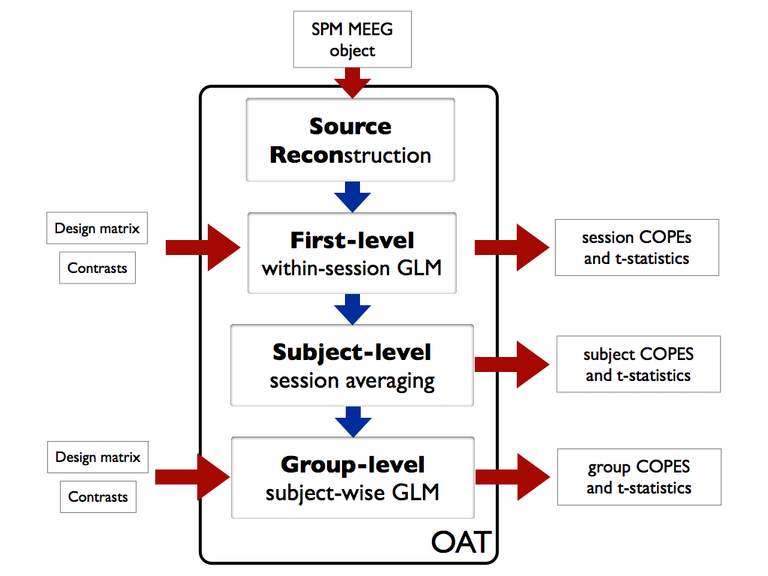
Since we are only analyzing a single session for a single subject here, we will only use the first two stages.
For more information about OAT see: https://ohba-analysis.github.io/osl-docs/pages/docs/oat.html
INITIALISE GLOBAL SETTINGS FOR THIS ANALYSIS
This cell sets the directory that OAT will work in. Change the workingdir variable to correspond to the correct directory on your computer before running the cell.
% directory where the data is:
datadir = fullfile(osldir,'example_data','faces_singlesubject','spm_files');

% directory to put the analysis in
workingdir = fullfile(osldir,'example_data','faces_singlesubject');
SET UP THE SUBJECTS FOR THE ANALYSIS
Specify a list of the SPM input files. Note that here we only have 1 subject, but more generally there would be more than one. For example:
spm_files_continuous{1} = [workingdir '/sub1_face_sss.mat'];
spm_files_continuous{2} = [workingdir '/sub2_face_sss.mat'];
etc...
% clear old spm files
clear spm_files_continuous spm_files_epoched

spm_files_continuous{1} = fullfile(datadir,'Aface_meg1.mat');
spm_files_epoched{1}    = fullfile(datadir,'eAface_meg1.mat');
SETUP SENSOR SPACE SOURCE RECON
This stage sets up the source reconstruction stage of an OAT analysis. The source_recon stage is always run even for a sensorspace analysis, though in these cases it simply prepares the data for subsequent analysis. In this example we define our input files (D_continuous and D_epoched) and conditions before setting a time frequency window from -200ms before stimulus onset to 400ms after and from 4Hz to 100Hz. The source recon method is set to 'none' as we are performing a sensorspace analysis. The oat.source_recon.dirname is where all the analysis will be stored. This includes all the intermediate steps, diagnostic plots and final results.
oat=[];
oat.source_recon.D_epoched=spm_files_epoched; % this is passed in so that the bad trials and bad channels can be read out
oat.source_recon.D_continuous=spm_files_continuous;
oat.source_recon.conditions={'Motorbike','Neutral face','Happy face','Fearful face'};
oat.source_recon.freq_range=[4 100]; % frequency range in Hz
oat.source_recon.time_range=[-0.2 0.4];
oat.source_recon.method='none';
oat.source_recon.normalise_method='none';

% Ensure that the directory name is unique (results in existing directories
% will be overwritten).
oat.source_recon.dirname = fullfile(workingdir,'sensorspace_erf');
SETUP THE FIRST LEVEL GLM
This cell defines the GLM parameters for the first level analysis. Critically this includes the design matrix (in Xsummary) and the contrast matrix. Xsummary is a parsimonious description of the design matrix. It contains values Xsummary{reg,cond}, where reg is a regressor index number and cond indexes different experimental conditions (e.g. pictures of faces, pictures of motorbikes). This will be used (by expanding the conditions over trials) to create the (num_regressors x num_trials) design matrix.
Each contrast is a vector containing a weight per condition defining how the condition parameter estimates are to be compared. Each vector will produce a different t-map across the sensors. Contrasts 1 and 2 describe positive correlations between each sensor's activity and the presence of a motorbike or face stimulus respectively. Contrast 3 tests whether each sensor's activity is larger for faces than motorbikes.
Xsummary={};
Xsummary{1}=[1 0 0 0];
Xsummary{2}=[0 1 0 0];
Xsummary{3}=[0 0 1 0];
Xsummary{4}=[0 0 0 1];
oat.first_level.design_matrix_summary=Xsummary;

% contrasts to be calculated:
oat.first_level.contrast={};
oat.first_level.contrast{1}=[3 0 0 0]'; % motorbikes
oat.first_level.contrast{2}=[0 1 1 1]'; % faces
oat.first_level.contrast{3}=[-3 1 1 1]'; % faces-motorbikes
oat.first_level.contrast_name{1}='motorbikes';
oat.first_level.contrast_name{2}='faces';
oat.first_level.contrast_name{3}='faces-motorbikes';

oat.first_level.cope_type='cope';
oat.first_level.report.first_level_cons_to_do=[2 1 3];
oat.first_level.bc=[0 0 0];

oat = osl_check_oat(oat);
Detected Elekta Neuromag 306 data. Using default Elekta Neuromag 306 settings.
Warning: oat.source_recon.modalities not set, or not set properly. Will set to
default:MEGPLANARMEGMAG
Using oat.source_recon.freq_range for oat.first_level.tf_freq_range
oat.source_recon.D_epoched set. OAT will do an epoched data trial-wise GLM
VIEW OAT SETTINGS
As well as using the settings we specified in the previous cell, calling osl_check_oat has filled in a bunch of other settings as well.
oat
oat.source_recon
oat.first_level
oat =

  struct with fields:

            to_do: [1 1 1 1]
         do_plots: 0
     source_recon: [1×1 struct]
      first_level: [1×1 struct]
    subject_level: [1×1 struct]
      group_level: [1×1 struct]
     osl2_version: '4f0b460'


ans =

  struct with fields:

                time_range: [-0.2000 0.4000]
                conditions: {1×4 cell}
              D_continuous: {'/Users/andrew/toolboxes/osl/example_data/faces_singlesubject/spm_files/Aface_meg1.mat'}
                 D_epoched: {'/Users/andrew/toolboxes/osl/example_data/faces_singlesubject/spm_files/eAface_meg1.mat'}
                freq_range: [4 100]
                   dirname: '/Users/andrew/toolboxes/osl/example_data/faces_singlesubject/sensorspace_erf'
            sessions_to_do: 1
                 epochinfo: []
                    method: 'none'
     bandstop_filter_mains: 0
        artefact_chanlabel: []
                modalities: {'MEGPLANAR'  'MEGMAG'}
             session_names: {'session1'}
          normalise_method: 'none'
                     regpc: 0
                  gridstep: 7
               forward_meg: 'Single Shell'
                       mri: []
                   pca_dim: 50
             force_pca_dim: 0
                      type: 'Scalar'
            hmm_num_states: 0
            hmm_num_starts: 1
               hmm_pca_dim: 40
    hmm_av_class_occupancy: 35
                    report: [1×1 struct]


ans =

  struct with fields:

                                     doGLM: 1
                     design_matrix_summary: {1×4 cell}
                                  contrast: {1×3 cell}
                             contrast_name: {1×3 cell}
                            sessions_to_do: 1
                                time_range: [-0.2000 0.4000]
                         baseline_timespan: [-0.2000 0]
                  do_weights_normalisation: 1
                            use_robust_glm: 0
                                        bc: [0 0 0]
              sensor_space_combine_planars: 'combine_cartesian'
                              bc_trialwise: 0
                                      name: 'first_level'
                   time_moving_av_win_size: []
          post_glm_time_moving_av_win_size: []
                      hmm_do_glm_statewise: 0
                                 tf_method: 'none'
                             tf_freq_range: [4 100]
                              tf_num_freqs: 1
                              time_average: 0
                     tf_multitaper_ncycles: []
      post_movingaverage_downsample_factor: []
                 post_tf_downsample_factor: []
                       tf_hilbert_freq_res: 2
    tf_hilbert_do_bandpass_for_single_freq: 0
                    tf_hilbert_freq_ranges: []
                          tf_morlet_factor: 6
                        tf_hanning_ncycles: []
                                 cope_type: 'cope'
                       save_trialwise_data: 0
                       trialwise_directory: []
                              parcellation: [1×1 struct]
                                is_epoched: 1
                             do_glm_demean: 0
                                    report: [1×1 struct]
                               warp_fields: []
CHECK OVER OAT SETTINGS
The osl_check_oat.m function should be used to setup the settings for these three stages of the pipeline.
to see what the mandatory fields are. Note that you MUST specify:
- oat.source_recon.time_range
- oat.source_recon.conditions
- oat.source_recon.D_continuous
- oat.source_recon.D_epoched
Descriptions of what these correspond to are also displayed when you type help osl_check_oat in to the matlab console.
We are only interested in the first two stages of an OAT analysis, as we are not doing any group analysis here:
- oat.source_recon
- oat.first_level
Each of these contains the settings for the relevant stages of the pipeline. You can read the Pipeline Stages section of the OSL manual to get more description about these two stages.
Take a look at oat.source_recon.dirname. This will be the name of the directory (full path) where the OAT will be stored, and is given a .oat extension. [Note that each OAT directory is associated with a specific source recon; a new source recon will overwrite an old directory if the same oat.source_recon.dirname is used, and the old source recon results will be lost. Hence, you should ensure that you change oat.source_recon.dirname for a new source recon analysis, if you want to avoid overwriting an old one.]
RUN OAT
The OAT structure you have created, oat, should be passed to the function osl_run_oat, to run the pipeline. However, the OAT structure should contain a structure (oat.to_do), which is a list of binary values indicating which part of the pipeline is to be run. E.g. oat.to_do=[1 1 0 0]; will run just the source recon and first level stages, whereas oat.to_do=[1 1 1 1]; will run all four (source-recon, first level, subject-level and group level). Here we are not doing any group analysis, so we need:
oat.to_do=[1 1 0 0];
OAT will produce and close a number of figures as it processes, we will discuss what they mean once it has finished (this takes a couple of minutes)
oat.to_do=[1 1 0 0];
oat = osl_run_oat(oat);
Detected Elekta Neuromag 306 data. Using default Elekta Neuromag 306 settings.
Warning: oat.source_recon.modalities not set, or not set properly. Will set to
default:MEGPLANARMEGMAG
oat.source_recon.D_epoched set. OAT will do an epoched data trial-wise GLM
*************************************************************
Running source_recon
*************************************************************
%%%%%%%%%%%%%%%%%%%%%%%%%%%%%%%%%%%%%%%%%%%%%%%%%%%%%%%%%%%%%%%%%%%%%%%%%%%%%%%%%%%%%%%%%%%%%%
%%%%%%%%%%%%%%%%%%%%%%%  RUNNING OAT SOURCE RECON (SENSOR SPACE SETUP) ON SESS = 1  %%%%%%%%%%%%%%%%%%%%%%%
Using continuous data as input
Using epoched data as input
Preparing source recon stage for /Users/andrew/toolboxes/osl/example_data/faces_singlesubject/spm_files/Aface_meg1.mat
Will be designated session1

SPM12: spm_eeg_copy (v7132)                        12:32:29 - 06/11/2019
========================================================================

SPM12: spm_eeg_copy (v7132)                        12:32:32 - 06/11/2019
========================================================================
Temporal filtering...

SPM12: spm_eeg_filter (v7125)                      12:32:35 - 06/11/2019
========================================================================
Filter bandpass (but, twopass)          :                    [4  100] Hz
Completed                               :          12:32:45 - 06/11/2019
Epoching...
Doing no within-trial baseline correction at the point of epoching

SPM12: spm_eeg_epochs (v7125)                      12:32:45 - 06/11/2019
========================================================================
Data type is missing or incorrect, assigning default.
Baseline correction                     :                              0
Number of trials                        :                            360
Completed                               :          12:32:54 - 06/11/2019
Changing the number of channels, so discarding online montages.

SPM12: spm_eeg_copy (v7132)                        12:33:05 - 06/11/2019
========================================================================
Saving source recon (sensorspace setup) results: session1_recon
*************************************************************
Running first_level
*************************************************************
%%%%%%%%%%%%%%%%%%%%%%%%%%%%%%%%%%%%%%%%%%%%%%%%%%%%%%%%%%%%%%%%%%%%%%%%%%%%%%%%%%%%%%%%%%%%%%
%%%%%%%%%%%%%%%%%%%%%%%  RUNNING OAT FIRST LEVEL ON SESS = 1  %%%%%%%%%%%%%%%%%%%%%%%

ans =

    '/Users/andrew/toolboxes/osl/example_data/faces_singlesubject/sensorspace_erf.oat/efsession1_spm_meeg.mat'


SPM12: spm_eeg_copy (v7132)                        12:33:15 - 06/11/2019
========================================================================

ans =

    '/Users/andrew/toolboxes/osl/example_data/faces_singlesubject/sensorspace_erf.oat/efsession1_spm_meeg_firstlevel.mat'

Working in sensor space
TIME DOMAIN, NOT DOWNSAMPLING; raw data at 250Hz, GLM at 250Hz.
Reconstruct time courses and computing stats for dataset session1_recon
CAREFUL: are you sure you want no first_level.do_glm_demean flag on with no constant regressors in the design matrix!!!!?
State 1 is active for 213.6secs
First level COPEs outputted will have dimension Nvoxels x Ntpts x Ncontrasts x Nfreqs:
306  151    3    1
size(sens_data_tf)=[325 151 356 1], (nsens x ntpts x ntri x nfreq)
 - estimated time to finish is 0 seconds
reading layout from file /Users/andrew/toolboxes/osl/layouts/neuromag306planar3.lay
reading layout from file /Users/andrew/toolboxes/osl/layouts/neuromag306planar2.lay
reading layout from file /Users/andrew/toolboxes/osl/layouts/neuromag306mag.lay
reading layout from file /Users/andrew/toolboxes/osl/layouts/neuromag306cmb.lay
Warning: Gradiometers combined with ERF and COPE: gradiometer COPEs will be
rectified
Changing the number of channels, so discarding online montages.
Changing the number of channels, so discarding online montages.
Saving statistics in file /Users/andrew/toolboxes/osl/example_data/faces_singlesubject/sensorspace_erf.oat/session1_first_level
Changing the number of channels, so discarding online montages.
Changing the number of channels, so discarding online montages.
reading layout from file /Users/andrew/toolboxes/osl/layouts/neuromag306cmb.lay
reading layout from file /Users/andrew/toolboxes/osl/layouts/neuromag306cmb.lay
Changing the number of channels, so discarding online montages.
Changing the number of channels, so discarding online montages.
reading layout from file /Users/andrew/toolboxes/osl/layouts/neuromag306cmb.lay
reading layout from file /Users/andrew/toolboxes/osl/layouts/neuromag306cmb.lay
Changing the number of channels, so discarding online montages.
Changing the number of channels, so discarding online montages.
reading layout from file /Users/andrew/toolboxes/osl/layouts/neuromag306cmb.lay
reading layout from file /Users/andrew/toolboxes/osl/layouts/neuromag306cmb.lay
View first level report at:
/Users/andrew/toolboxes/osl/example_data/faces_singlesubject/sensorspace_erf.oat/plots/first_level/sess_session1_MEGPLANAR/report.html
To view OAT report, point your browser to <a href="/Users/andrew/toolboxes/osl/example_data/faces_singlesubject/sensorspace_erf.oat/plots/report.html">/Users/andrew/toolboxes/osl/example_data/faces_singlesubject/sensorspace_erf.oat/plots/report.html</a>
VIEW RESULTS
OAT runs the GLM for every time point and frequency band across all sensors.
OAT will create a report containing a summary of the first level analysis results (as well as some diagnostic figures from the source reconstruction). The specific content of this report depends upon settings in oat.first_level.report:
- oat.first_level.report.modality_to_do - e.g. MEGPLANAR, MEGMAG (only in sensor space)
- oat.first_level.report.first_level_cons_to_do; - plots only these contrasts and uses first one in list to determine max vox, time, freq
- oat.first_level.report.time_range; - to determine max vox, time, freq
- oat.first_level.report.freq_range; - to determine max vox, time, freq
Open the report indicated in oat.results.report in a web browser (there will also be a link to this available in the Matlab output). This displays the diagnostic plots.
- At the top of the file is a link to oat.results.logfile (a file containing the matlab output) - you should check this for any errors or unusual warnings.
- Then there will be a list of reports for each OAT stage.
- Click on the "First level (epoched)" link to bring up the first level reports.
This brings up a list of sessions. Here we have only preprocessed one session. Click on the "Session 1 report" link to bring up the diagnostic plots for session 1 and take a look.
The settings in the current OAT will generate several images
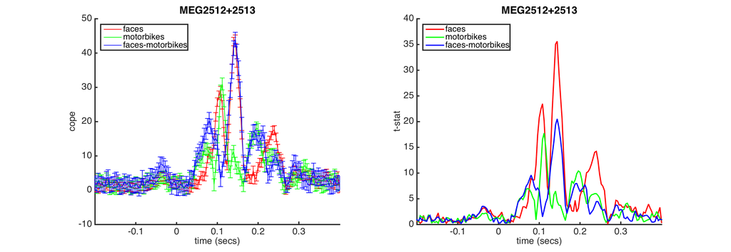
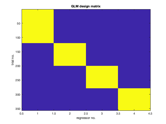
- Design Matrix - the design matrix used in the GLM analysis
- COPE and T-stat plots - All three contrasts are shown with COPE on the left and the t-stat on the right. These are from the peak sensor for the faces contrast.
- Topo and ERF plots - These are shown for each of the contrasts. The topoplot shows the response at the peak time point for the faces contrast and the ERF plot shows the response across the whole epoch.
disp(oat.results.report.html_fname); % show path to web page report
/Users/andrew/toolboxes/osl/example_data/faces_singlesubject/sensorspace_erf.oat/plots/report.html
OAT RESULTS STRUCTURE
Run the following code to see what oat.results contains. This includes:
- oat.results.logfile - (a file containing the matlab output)
- oat.results.report - (a file corresponding to a web page report with diagnostic plots)
It is highly recommended that you always inspect the oat.results.report, to ensure that OAT has run successfully.
Open the report indicated in oat.results.report in a web browser (there will also be a link to this available in the Matlab output). This displays the diagnostic plots.
- At the top of the file is a link to oat.results.logfile (a file containing the matlab output) - you should check this for any errors or unusual warnings.
- Then there will be a list of reports for each OAT stage.
Click on the "First level (epoched)" link to bring up the first level reports.
This brings up a list of sessions. Here we have only preprocessed one session. Click on the "Session 1 report" link to bring up the diagnostic plots for session 1 and take a look.
The results can be loaded back into matlab using oat_load_results. This is useful for checking over results of the GLM or as the basis for further analyses.
% Show OAT results
disp('oat.results:');
disp(oat.results);
oat.results:
        date: '06-Nov-2019'
    plotsdir: '/Users/andrew/toolboxes/osl/example_data/faces_singlesubject/sensorspace_erf.oat/plots'
     logfile: '/Users/andrew/toolboxes/osl/example_data/faces_singlesubject/sensorspace_erf.oat/plots/log-06-Nov-2019.txt'
      report: [1×1 struct]
VIEW THE GLM DESIGN MATRIX
Running the OAT analysis will create an OAT output directory (whose name is the name set in oat.source_recon.dirname with a ?.oat? suffix added). This contains all you need to access the results of the analysis. It contains the analysis settings and the pointers to files containing the results for each of the pipeline stages that have been run. The oat can be loaded into Matlab with the call:
oat=osl_load_oat(oat.source_recon.dirname);
Each stage of the OAT pipeline will also have stored its results in a .mat data file saved in the OAT output directory. Note that for source_recon and first_level these are saved separately for each subject. The names of these files are stored in the corresponding part of the OAT structure, e.g.
- oat.source_recon.results_fnames
- oat.first_level.results_fnames
- oat.subject_level.results_fnames
- oat.group_level.results_fnames
These can loaded into Matlab, e.g. to load session 1's source reconstruction results use the call:
recon_results = oat_load_results(oat,oat.source_recon.results_fnames{1})
E.g. to load session 2's first level stats results, you can use the call:
stats = oat_load_results(oat,oat.first_level.results_fnames{2})
Run the following code to load in the stats results from the GLM you just ran and plot the design matrix. This is the nconditions x ntrials design matrix which is used to fit the GLM (NOTE that column 1 is motorbikes, columns 2-4 are faces)
% load first-level GLM result
stats1=oat_load_results(oat,oat.first_level.results_fnames{1});

% Plot design matrix
figure;imagesc(stats1.x);title('GLM design matrix');xlabel('regressor no.');ylabel('trial no.');
VISUALISE USING FIELDTRIP
A lot of the visualisations work using functions from fieldtrip. These offer a wide range of visualisation options and are highly customisable. Here we will use an OSL function which plots an OAT result in a fieldtrip multiplot.
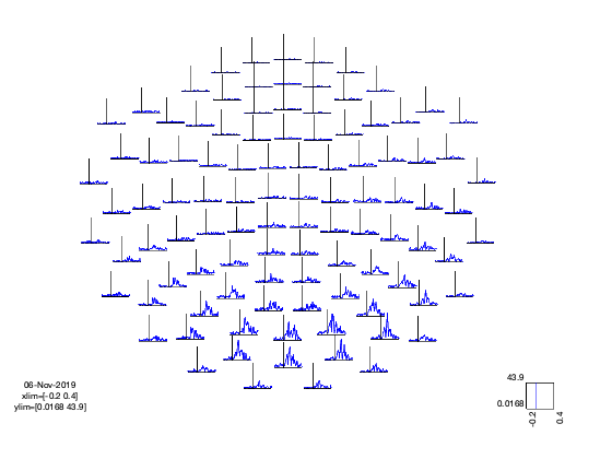
We will plot the COPE time-courses for the faces-motorbikes contrast across all the Planar Gradiometers by defining the following options and calling oat_stats_multiplotER.
Note that this produces an interactive figure, with which you can:
- click and drag to draw a box around a set of sensors
- click in the drawn box to produce a plot of the time series
- on the time series plot you can draw a time window
- and click in the window to create a topoplot averaged over that time window (which is itself interactive....!)
S2=[];
S2.oat=oat;
S2.stats_fname=oat.first_level.results_fnames{1};
S2.modality='MEGPLANAR'; % can also set this to 'MEGMAG'
S2.first_level_contrast=[3]; % view faces-motorbikes contrast
S2.view_cope=1; % set to 0 to see the t-stat

% calculate t-stat using contrast of absolute value of parameter estimates
[cfg, dats, fig_handle]=oat_stats_multiplotER(S2);
Changing the number of channels, so discarding online montages.
Changing the number of channels, so discarding online montages.
reading layout from file /Users/andrew/toolboxes/osl/layouts/neuromag306cmb.lay