OAT 3 - Sourcespace Analysis

This practical will work with a single subject's data from an emotional faces experiment (Elekta Neuromag data).

Work your way through the script cell by cell using the supplied dataset. As well as following the instructions below, make sure that you read all of the comments and understand each step as you go.

We will estimate neural activity in the brain's source space using a beamformer algorithm, task dependant differences in this source activity is then quantified using a GLM. This will go through the following steps:

This practical requires the first part of the osl_example_coregistration practical to be run first. If you haven't run this before, please do so before starting this session.

Contents

INITIALISE GLOBAL SETTINGS FOR THIS ANALYSIS

This cell sets the directory that OAT will work in. Change the workingdir variable to correspond to the correct directory on your computer before running the cell.

% directory where the data is:
datadir = fullfile(osldir,'example_data','faces_singlesubject','spm_files');
structdir =  fullfile(osldir,'example_data','faces_singlesubject','structurals');

% directory to put the analysis in
workingdir = fullfile(osldir,'example_data','faces_subject1_data_osl2');

SET UP THE SUBJECTS FOR THE ANALYSIS

Specify a list of the SPM input files. Note that here we only have 1 subject, but more generally there would be more than one. For example:

spm_files_continuous{1} = [workingdir '/sub1_face_sss.mat'];

spm_files_continuous{2} = [workingdir '/sub2_face_sss.mat'];

etc...

% clear old spm files
clear spm_files_continuous spm_files_epoched

spm_files_continuous{1}=fullfile(datadir,'Aface_meg1.mat');
spm_files_epoched{1}=fullfile(datadir,'eAface_meg1.mat');

% Update the location of the structural files within the MEEG files
D = spm_eeg_load(spm_files_continuous{1});
D = osl_update_inv_dir(D,structdir);
D.save()

D = spm_eeg_load(spm_files_epoched{1});
D = osl_update_inv_dir(D,structdir);
D.save()

SPM M/EEG data object
Type: continuous
Transform: time
1 conditions
323 channels
218000 samples/trial
1 trials
Sampling frequency: 250 Hz
Loaded from file  /Users/andrew/toolboxes/osl/example_data/faces_singlesubject/spm_files/Aface_meg1.mat

Use the syntax D(channels, samples, trials) to access the data
Type "methods('meeg')" for the list of methods performing other operations with the object
Type "help meeg/method_name" to get help about methods

SPM M/EEG data object
Type: single
Transform: time
4 conditions
323 channels
751 samples/trial
360 trials
Sampling frequency: 250 Hz
Loaded from file  /Users/andrew/toolboxes/osl/example_data/faces_singlesubject/spm_files/eAface_meg1.mat

Use the syntax D(channels, samples, trials) to access the data
Type "methods('meeg')" for the list of methods performing other operations with the object
Type "help meeg/method_name" to get help about methods

SETUP THE OAT:

The oat.source_recon options define the parameters for the data filtering, windowing and beamforming. We define the continuous and epoched SPM MEEG object files, conditions and time-frequency options in the same way as the sensorspace OAT. The In this section we will do a wholebrain beamformer, followed by a trial-wise GLM that will correspond to a comparison of the ERFs for the different conditions. The source-space projection is defined by a new set of options.

The critical options are:

These options are the same as the sensorspace OAT and define input-data, conditions, filtering and windowing.

oat=[];
oat.source_recon.D_continuous=spm_files_continuous;
oat.source_recon.D_epoched=spm_files_epoched;

oat.source_recon.conditions={'Motorbike','Neutral face','Happy face','Fearful face'};
oat.source_recon.freq_range=[3 40]; % frequency range in Hz
oat.source_recon.time_range=[-0.2 0.4]; % time range in secs

These options specify the source reconstruction that will take place.

oat.source_recon.method='beamform';
oat.source_recon.normalise_method='mean_eig';
oat.source_recon.gridstep=8; % in mm
oat.source_recon.forward_meg='Single Shell';
oat.source_recon.modalities{1}={'MEGPLANAR', 'MEGMAG'};
oat.source_recon.report.do_source_variance_maps=1;

oat.source_recon.dirname=fullfile(workingdir,'beamformer_erf'); % directory the oat and results will be stored in

SPECIFIY FIRST LEVEL OPTIONS

These options are the same as the sensorspace ERF tutorial.

design_matrix_summary is a parsimonious description of the design matrix. It contains values design_matrix_summary{reg,cond}, where reg is a regressor index number and cond indexes different experimental conditions (e.g. pictures of faces, pictures of motorbikes). This will be used (by expanding the conditions over trials) to create the (num_regressors x num_trials) design matrix.

design_matrix_summary={};
design_matrix_summary{1}=[1 0 0 0];design_matrix_summary{2}=[0 1 0 0];design_matrix_summary{3}=[0 0 1 0];design_matrix_summary{4}=[0 0 0 1];
oat.first_level.design_matrix_summary=design_matrix_summary;

% contrasts to be calculated:
oat.first_level.contrast={};
oat.first_level.contrast{1}=[3 0 0 0]'; % motorbikes
oat.first_level.contrast{2}=[0 1 1 1]'; % faces
oat.first_level.contrast{3}=[-3 1 1 1]'; % faces-motorbikes
oat.first_level.contrast_name={};
oat.first_level.contrast_name{1}='motorbikes';
oat.first_level.contrast_name{2}='faces';
oat.first_level.contrast_name{3}='faces-motorbikes';
oat.first_level.report.first_level_cons_to_do=[2 1 3];

oat.first_level.time_range=[-0.1 0.3];
oat.first_level.post_tf_downsample_factor=1;
oat.first_level.name=['wholebrain_first_level'];

oat = osl_check_oat(oat);

Detected Elekta Neuromag 306 data. Using default Elekta Neuromag 306 settings.
Warning: oat.source_recon.modalities not set, or not set properly. Will set to
default:MEGPLANARMEGMAG 
Using oat.source_recon.freq_range for oat.first_level.tf_freq_range
oat.source_recon.D_epoched set. OAT will do an epoched data trial-wise GLM

RUN THE OAT:

We only need to run the source_recon and first_level stages in this tutorial, so the oat.to_do flags for the subject_level and group_level OAT stages are set to 0.

The OAT will produce and close a number of figures as it processes, we will discuss what they mean once it has finished (this takes a couple of minutes)

oat.to_do=[1 1 0 0];
oat = osl_run_oat(oat);

close all % close any open figures

Detected Elekta Neuromag 306 data. Using default Elekta Neuromag 306 settings.
Warning: oat.source_recon.modalities not set, or not set properly. Will set to
default:MEGPLANARMEGMAG 
oat.source_recon.D_epoched set. OAT will do an epoched data trial-wise GLM
*************************************************************
Running source_recon
*************************************************************

mask_fname =

    '/Users/andrew/toolboxes/osl/std_masks/MNI152_T1_8mm_brain.nii.gz'

Using whole brain
Using beamform for source reconstruction
%%%%%%%%%%%%%%%%%%%%%%%%%%%%%%%%%%%%%%%%%%%%%%%%%%%%%%%%%%%%%%%%%%%%%%%%%%%%%%%%%%%%%%%%%%%%%%
%%%%%%%%%%%%%%%%%%%%%%%  RUNNING OAT SOURCE RECON ON SESS = 1  %%%%%%%%%%%%%%%%%%%%%%%
Using continuous data as input
Using epoched data as input
Preparing source recon stage for /Users/andrew/toolboxes/osl/example_data/faces_singlesubject/spm_files/Aface_meg1.mat
Will be designated session1

SPM12: spm_eeg_copy (v7132)                        14:47:34 - 06/11/2019
========================================================================

SPM12: spm_eeg_copy (v7132)                        14:47:37 - 06/11/2019
========================================================================
Temporal filtering...

SPM12: spm_eeg_filter (v7125)                      14:47:40 - 06/11/2019
========================================================================
Filter bandpass (but, twopass)          :                     [3  40] Hz
Completed                               :          14:47:51 - 06/11/2019
Epoching...
Doing no within-trial baseline correction at the point of epoching

SPM12: spm_eeg_epochs (v7125)                      14:47:51 - 06/11/2019
========================================================================
Data type is missing or incorrect, assigning default.
Baseline correction                     :                              0
Number of trials                        :                            360
Completed                               :          14:48:00 - 06/11/2019
Warning: S.modalities not set. Will set to default 

No kicks found in the eigenspectrum. Estimated dimensionality has been kept at 50.
Dimensionality for modality MEGPLANAR is: 50
Modality MEGPLANAR has smallest sqrt(eig) = 8.7897

No kicks found in the eigenspectrum. Estimated dimensionality has been kept at 50.
Dimensionality for modality MEGMAG is: 50
Modality MEGMAG has smallest sqrt(eig) = 300.2156
Modality MEGPLANAR has data normalisation 8.7897
Modality MEGMAG has data normalisation 300.2156
No new channels information : setting channels info automatically.

No kicks found in the eigenspectrum. Estimated dimensionality has been kept at 50.
Overall dimensionality is: 49

No kicks found in the eigenspectrum. Estimated dimensionality has been kept at 50.
Dimensionality for modality MEGPLANAR is: 50
Modality MEGPLANAR has smallest sqrt(eig) = 1

No kicks found in the eigenspectrum. Estimated dimensionality has been kept at 50.
Dimensionality for modality MEGMAG is: 50
Modality MEGMAG has smallest sqrt(eig) = 1
Changing the number of channels, so discarding online montages.

SPM12: spm_eeg_copy (v7132)                        14:49:02 - 06/11/2019
========================================================================
Co-registration and setting up forward model...

SPM12: spm_eeg_inv_forward (v7354)                 14:49:05 - 06/11/2019
========================================================================
Warning: A value of class "int32" was indexed with no subscripts specified.
Currently the result of this operation is the indexed value itself, but in a
future release, it will be an error. 
Warning: A value of class "int32" was indexed with no subscripts specified.
Currently the result of this operation is the indexed value itself, but in a
future release, it will be an error. 
Warning: A value of class "int32" was indexed with no subscripts specified.
Currently the result of this operation is the indexed value itself, but in a
future release, it will be an error. 
Warning: A value of class "int32" was indexed with no subscripts specified.
Currently the result of this operation is the indexed value itself, but in a
future release, it will be an error. 
Warning: A value of class "int32" was indexed with no subscripts specified.
Currently the result of this operation is the indexed value itself, but in a
future release, it will be an error. 
Completed                               :          14:49:05 - 06/11/2019
BF working directory: /Users/andrew/toolboxes/osl/example_data/faces_subject1_data_osl2/beamformer_erf.oat


------------------------------------------------------------------------
06-Nov-2019 14:49:08 - Running job #1
------------------------------------------------------------------------
06-Nov-2019 14:49:08 - Running 'Prepare data'
06-Nov-2019 14:49:08 - Done    'Prepare data'
06-Nov-2019 14:49:08 - Running 'Define sources'
computing surface normals
06-Nov-2019 14:49:33 - Done    'Define sources'
06-Nov-2019 14:49:33 - Running 'Covariance features'
Ignoring job.woi. Using Class channel in D object to determine the time samples to use
06-Nov-2019 14:49:35 - Done    'Covariance features'
06-Nov-2019 14:49:35 - Running 'Inverse solution'
06-Nov-2019 14:49:38 - Done    'Inverse solution'
06-Nov-2019 14:49:38 - Running 'Output'
06-Nov-2019 14:49:42 - Done    'Output'
06-Nov-2019 14:49:42 - Running 'Write'

SPM12: spm_eeg_montage (v7169)                     14:49:43 - 06/11/2019
========================================================================
Completed                               :          14:49:45 - 06/11/2019

SPM12: spm_eeg_montage (v7169)                     14:49:47 - 06/11/2019
========================================================================
Completed                               :          14:49:50 - 06/11/2019
06-Nov-2019 14:49:54 - Done    'Write'
06-Nov-2019 14:49:54 - Done

Saving source-space results: session1_recon
Processing trial 360 of 360 - estimated time to finish is 0 seconds
View source recon report at:
<a href="/Users/andrew/toolboxes/osl/example_data/faces_subject1_data_osl2/beamformer_erf.oat/plots/06-Nov-2019_source_recon/report.html">/Users/andrew/toolboxes/osl/example_data/faces_subject1_data_osl2/beamformer_erf.oat/plots/06-Nov-2019_source_recon/report.html</a>
*************************************************************
Running first_level
*************************************************************
%%%%%%%%%%%%%%%%%%%%%%%%%%%%%%%%%%%%%%%%%%%%%%%%%%%%%%%%%%%%%%%%%%%%%%%%%%%%%%%%%%%%%%%%%%%%%%
%%%%%%%%%%%%%%%%%%%%%%%  RUNNING OAT FIRST LEVEL ON SESS = 1  %%%%%%%%%%%%%%%%%%%%%%%

ans =

    '/Users/andrew/toolboxes/osl/example_data/faces_subject1_data_osl2/beamformer_erf.oat/efsession1_spm_meeg.mat'


SPM12: spm_eeg_copy (v7132)                        14:50:28 - 06/11/2019
========================================================================

ans =

    '/Users/andrew/toolboxes/osl/example_data/faces_subject1_data_osl2/beamformer_erf.oat/efsession1_spm_meeg_firstlevel.mat'

Using same indices as lower_level
TIME DOMAIN, NOT DOWNSAMPLING; raw data at 250Hz, GLM at 250Hz.
Reconstruct time courses and computing stats for dataset session1_recon
CAREFUL: are you sure you want no first_level.do_glm_demean flag on with no constant regressors in the design matrix!!!!?
State 1 is active for 213.6secs
First level COPEs outputted will have dimension Nvoxels x Ntpts x Ncontrasts x Nfreqs:
3559   100     3     1
size(sens_data_tf)=[325 151 356 1], (nsens x ntpts x ntri x nfreq)
 - estimated time to finish is 0 seconds
Saving statistics in file /Users/andrew/toolboxes/osl/example_data/faces_subject1_data_osl2/beamformer_erf.oat/session1_wholebrain_first_level
To create niftii files from this use a call to oat_save_nii_stats
Outputting nii files for first level contrast 2
Outputting nii files for first level contrast 1
Outputting nii files for first level contrast 3
E.g. to view nii file: 
fsleyes('/Users/andrew/toolboxes/osl/example_data/faces_subject1_data_osl2/beamformer_erf.oat/session1_wholebrain_first_level_dir/tstat3_2mm.nii.gz')
View first level report at:
/Users/andrew/toolboxes/osl/example_data/faces_subject1_data_osl2/beamformer_erf.oat/plots/wholebrain_first_level/sess_session1/report.html
To view OAT report, point your browser to <a href="/Users/andrew/toolboxes/osl/example_data/faces_subject1_data_osl2/beamformer_erf.oat/plots/report.html">/Users/andrew/toolboxes/osl/example_data/faces_subject1_data_osl2/beamformer_erf.oat/plots/report.html</a>

VIEW OAT REPORT

Once finished, OAT will print a link to a html report. Click to open it in the matlab html browser.

Source Recon

Firstly, click to open the "Session_1_report". This contains the plots relevent to the source_recon stage. This shows the results of the sensor normalisation that is done prior to the source reconstruction. This is done to ensure that all sensor types can contribute appropriately to the source reconstruction.

Note that the eigenspectrum of the sensordata ('Pre-normalised log eigenspectrum') drops off sharply at around 64, this indicates the rank of the sensor data which is limited by the maxfilter de-noising that was done during the preprocessing of this data.

The Pre-normalised variances shows the sensor-by-sensor variance across time. Channels 205-306 are the Magnetometers and have much higher variance than the Gradiometers. We need to normalise the data to remove this disparity or the information in the Magnetometers will dominate the reconstruction.

In the normalised_eigs plot below, we can see that the 'mean_eig' sensor normalisation has both removed the shelf in the eigenspectrum and brought the sensor variances in line with each other.

First Level

Click back to the first page and on to the 'First level (epoched) report' and then the 'session1 report'. This contains a results summary from the voxel-wise GLM

Design matrix plot. At the top is the design matrix used for each subject. Red values indicate a value of 1, blue indicates a value of zero. It is worth noting if every regressor (in this case corresponding to the four different conditions) is well represented. For example, if aggressive amounts of outlier rejection has been applied then it is possible to end up with very few trials in a regressor.

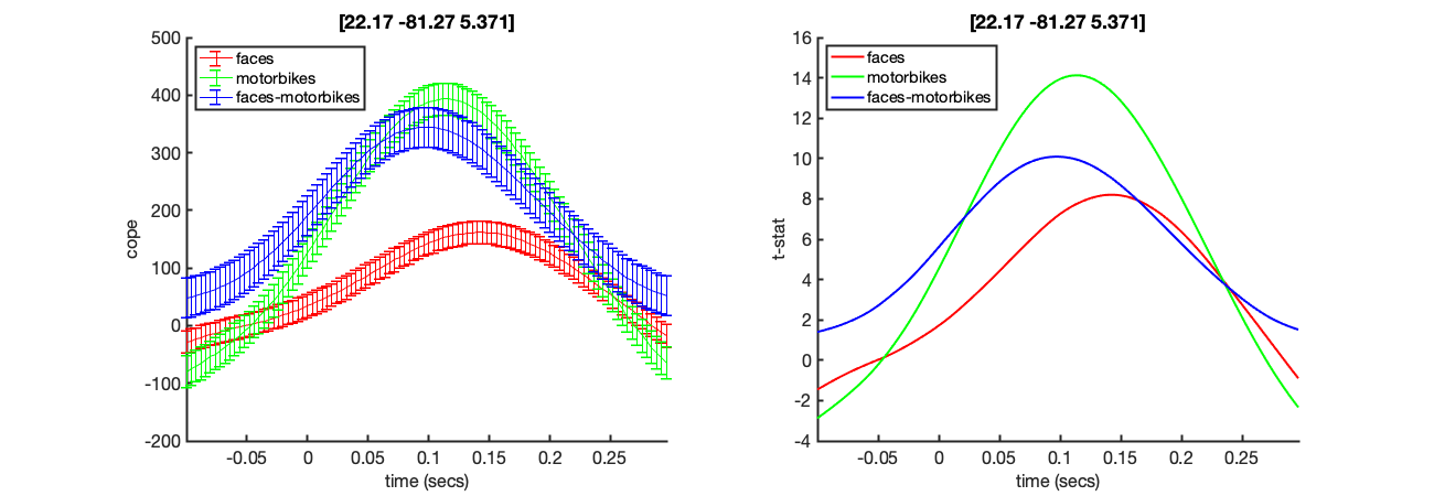
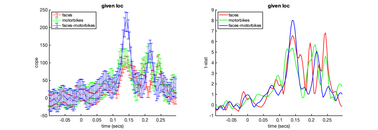
Stats plots These show the time courses of the COPEs and t-stats for the different contrasts listed in oat.first_level.report.first_level_cons_to_do, at the MNI coordinated indicated in the title of the plots. This MNI coordinate is chosen by finding the voxel with the maximum t-stat for the first contrast listed in oat.first_level.report.first_level_cons_to_do.

The COPE is on the left and the t-stat on the right. Note the large peak around 96ms after stimulus onset.

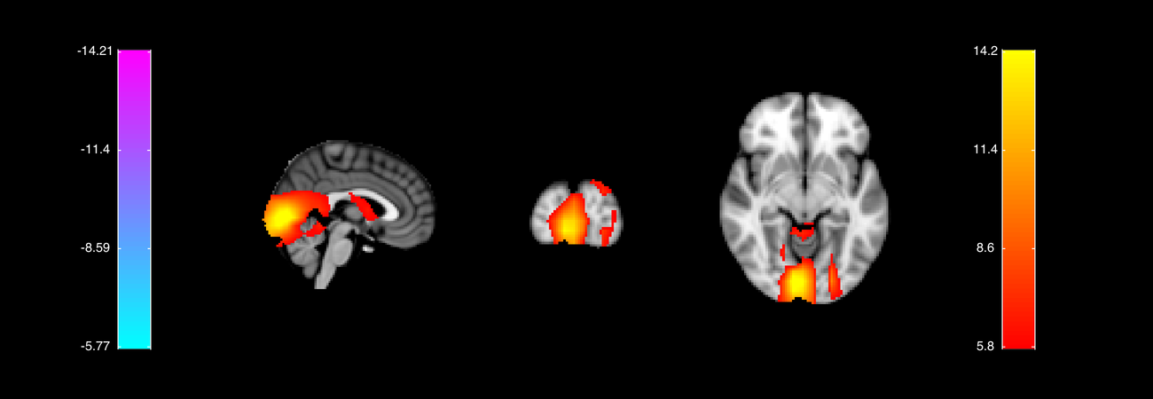
COPE and t-stat orthoview plots These show orthoviews of the COPEs and t-stats for the different contrasts listed in oat.first_level.report.first_level_cons_to_do, at the time point indicated in the title of the plots. This time point is chosen by finding the time point with the maximum t-stat for the first contrast listed in oat.first_level.report.first_level_cons_to_do.

This time-point is around 136ms and shows peaks in lateral and medial occipital cortex. These are right hemisphere lateralised for the Faces and Faces-Motorbikes condition.

OUTPUT SUBJECT'S NIFTII FILES

The html report gives a brief summary of the results but we would like to go into more detail.

We can do this by saving the contrast of parameter estimates (COPEs) and t-statistics for each of our contrasts to NIFTI images.

S2=[];
S2.oat=oat;
S2.stats_fname=oat.first_level.results_fnames{1};
S2.first_level_contrasts=[3,1,2];
S2.resamp_gridstep=oat.source_recon.gridstep;
[statsdir,times,count]=oat_save_nii_stats(S2);

Outputting nii files for first level contrast 3
Outputting nii files for first level contrast 1
Outputting nii files for first level contrast 2
E.g. to view nii file: 
fsleyes('/Users/andrew/toolboxes/osl/example_data/faces_subject1_data_osl2/beamformer_erf.oat/session1_wholebrain_first_level_dir/tstat2_8mm.nii.gz')

OPEN NIFTII RESULTS IN FSLVIEW

We can now view the nifti images containing our GLM results using osleyes.

o = osleyes(fullfile(statsdir,['tstat1_' num2str(oat.source_recon.gridstep) 'mm.nii.gz']));

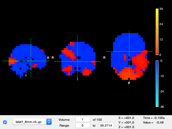
We need to tweak the viewing settings to see the results well.

Firstly, set the 'Min' and 'Max' colour limits to 15 and 25, respectively.

o.layer(2).clim = [15 25];

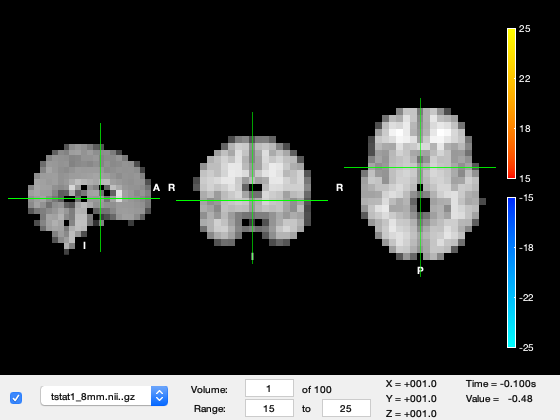
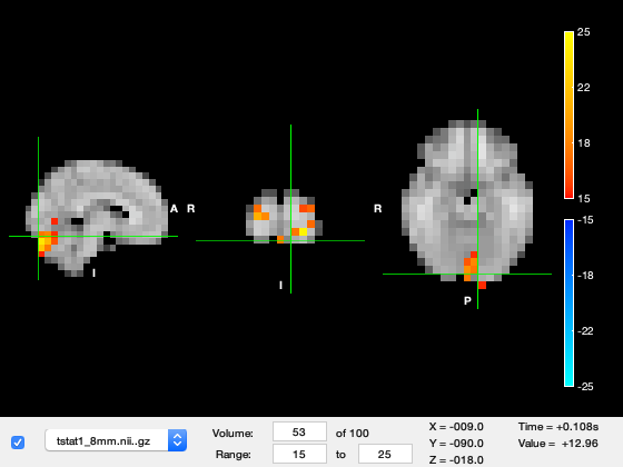
We are currently looking at the first time-point in the source_recon window which corresponds to -100ms, in which not much is happening. Change the 'Volume' to 49, which corresponds to around 100ms after stimulus onset. You should see a response in early visual cortex at the back of the brain. The time value now shows around 200ms, which is 100ms after stimulus onset.

o.layer(2).volume = 53;
o.current_point = [-9 -90 -18]; % set the location of the crosshair

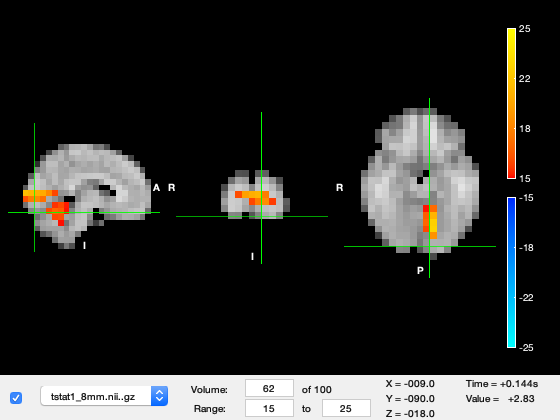
Now change the 'Volume' to 62, corresponding to around 140ms after stimulus onset. The peak of activation jumps to the right hemiphere visual cortex.

o.layer(2).volume = 62;

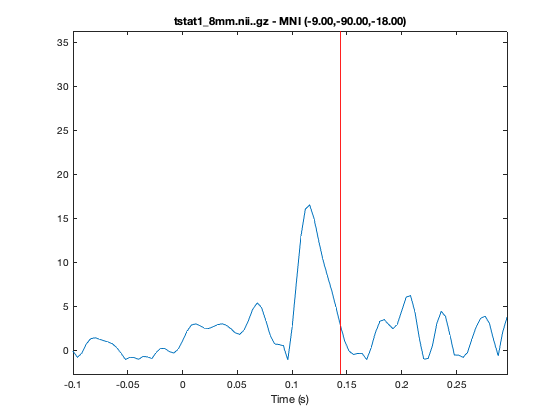
You can futher investigate the results by plotting the time series, by right clicking on the plot and selecting 'plot_timeseries' or using the 'plot_timeseries' method on the osleyes object. This will bring up a new window showing the t-value across time for the voxel under crosshair. The MNI coordinates are also displayed in the title of the plot. You can navigate across space by clicking on a part of the brain and time by clicking at a time-point on the timeseries.

o.plot_timeseries

Try changing to code in the previous cell to bring up the tstats for contrast 3 'Face-Motorbikes'. Following the same visualisation instructions you should be able to see that the early time-window (Volume 49) does not contain any large responses whereas the later response (Volume 59) still occurs. This indicates that there are no large differences between Faces and Motorbikes in the the early response, whereas the later response does differ.

INVESTIGATING LOCATION OF INTEREST USING AN MNI COORDINATE

We may want to see the results across all contrasts for a single ROI to gain another perspective on our results.

Here we will interrogate the wholebrain OAT (run above) using a specified MNI coordinate.

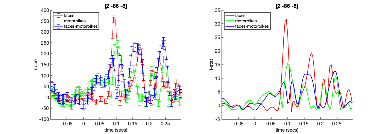
Run the code below now. This will bring up a the COPE and tstat estimates across time for a voxel in visual cortex. Note the prominant response around 100ms

Try changing the code to run at 32,-64,-18

This corresponds to a point in Right Hemisphere Fusiform Cortex. Note that the 100ms response does not appear here, rather the later Face specific response is more dominant.

mni_coord=[4,-82,-8]; % Visual Cortex Voxel

S2=[];
S2.vox_coord=mni_coord;
S2.stats=oat.first_level.results_fnames{1};
S2.oat=oat;
S2.first_level_cons_to_do=oat.first_level.report.first_level_cons_to_do; % plots all of these contrasts

[vox_ind_used] = oat_plot_vox_stats(S2);

Note that this output is a combination of all of the NIFTI files that could otherwise be viewed individually using osleyes. For example, to plot just the faces tstat for the same voxel shown above, we could use

o = osleyes(fullfile(statsdir,['tstat2_' num2str(oat.source_recon.gridstep) 'mm.nii.gz']));
o.current_point = mni_coord;
o.plot_timeseries;
close(o.fig); % Close the volume viewer, because we only want the time series plot

INVESTIGATING REGIONS OF INTEREST USING AN MNI MASK

In this section we will interrogate the wholebrain OAT (run above) using an ROI mask. Here we will use an MNI mask of the right temporal occipital fusiform cortex, to perform first level statistics restricted to the mask. The final result will correspond to a spatial average over the mask.

Unlike the virtual electrode, the results from many voxels (all defined in the binary mask in S2.mask_fname) are extracted and the average results across these points presented.

Apply a mask and spatially average the results over an ROI

S2=[];
S2.oat=oat;
S2.stats_fname=oat.first_level.results_fnames{1};
S2.mask_fname=fullfile(osldir,'example_data','faces_singlesubject','structurals',['Right_Temporal_Occipital_Fusiform_Cortex_' num2str(oat.source_recon.gridstep) 'mm.nii.gz']);
[stats,times,mni_coords_used]=oat_output_roi_stats(S2);

Plot the COPEs and t-stats within the ROI

S2=[];
S2.stats=stats;
S2.oat=oat;
S2.first_level_cons_to_do=oat.first_level.report.first_level_cons_to_do; % plots all of these contrasts
[vox_ind_used] = oat_plot_vox_stats(S2);

TIME-FREQUENCY ANALYSIS ACROSS A SOURCE-SPACE PARCELLATION

Often we want to interrogate neuronal responses in the frequency domain rather than the time-domain ERF. As we saw in the sensor-space practical we can extend the OAT to compute the GLM across a time-frequency decomposition of the data. Here we will extend the analysis to compute the first level GLM across a detailed time-frequency decomposition.

The GLM across the full time-frequency decomposition takes much longer to compute than the ERF or power within a single frequency band. As such we will run a time-frequency OAT across a 39 node source-space parcellation.

This has several benefits. Firstly, we can reduce noise by pooling across many voxels within a source parcel and secondly it is much faster to compute time-frequency transforms for 39 parcels than 306 Sensors or ~3500 Voxels. The details of source parcellations are covered in the ROInets practical sessions - for the moment we can consider the parcellation to be simple way to compute the OAT across many Regions of Interest at the same time.

Most of the OAT settings do not need to be changed for this analysis. We just need to define which parcellation should be applied and add the time-frequency decomposition parameters in the first level.

We are going to use the wholebrain OAT (which was run above), to make use of the settings and source_recon results already in there. The new time- frequency parameters are:

The new parcellation parameters are defined within a oat.first_level.parcellation struct. the critical parameters are:

LOAD PREVIOUSLY RUN OAT

We are going to use the wholebrain OAT (which was run above for the ERF analysis), to make use of the settings already in there

oat.source_recon.dirname=fullfile(workingdir,'beamformer_erf'); % Make sure this matches the dirname used above
oat.first_level.name=['wholebrain_first_level'];
oat=osl_load_oat(oat);

% Give the first level analysis a new name to avoid copying over previous
% first-level analyses:
oat.first_level.name=[oat.first_level.name '_parc' num2str(oat.first_level.parcellation.do)];

oat.source_recon.report.do_source_variance_maps=0;

% Add first level source recon options
oat.first_level.tf_freq_range=[4 30]; % frequency range in Hz
oat.first_level.time_range=[-0.1 0.3];
oat.first_level.tf_num_freqs=13;
oat.first_level.tf_method='morlet';
oat.first_level.post_tf_downsample_factor=1;

oat.first_level.report.time_range = [.08 .22];
oat.first_level.report.first_level_cons_to_do = [2,1,3];
oat.first_level.bc=[1 1 0]; % specifies whether or not baseline correction is done for the different contrasts

% Define the parameters for the parcellation
oat.first_level.parcellation.do=1;

% Path to the nifti defining the parcellation
parcellationfile=fullfile(osldir,'example_data','faces_singlesubject','structurals','fmri_d100_parcellation_with_PCC_reduced_2mm_ds8mm.nii.gz');

% Define the parcellation options.
oat.first_level.parcellation.parcellation=parcellationfile;
oat.first_level.parcellation.orthogonalisation = 'none';
oat.first_level.parcellation.method            = 'spatialBasis';

% Check and run the source_recon and first_level OAT stges
oat = osl_check_oat(oat);

% Rerun the first level OAT.
oat.to_do=[1 1 0 0];
oat = osl_run_oat(oat);

Loaded OAT: /Users/andrew/toolboxes/osl/example_data/faces_subject1_data_osl2/beamformer_erf.oat/oat_wholebrain_first_level_sub_level_group_level.mat
Detected Elekta Neuromag 306 data. Using default Elekta Neuromag 306 settings.
Warning: oat.source_recon.modalities not set, or not set properly. Will set to
default:MEGPLANARMEGMAG 
oat.source_recon.D_epoched set. OAT will do an epoched data trial-wise GLM
Detected Elekta Neuromag 306 data. Using default Elekta Neuromag 306 settings.
Warning: oat.source_recon.modalities not set, or not set properly. Will set to
default:MEGPLANARMEGMAG 
oat.source_recon.D_epoched set. OAT will do an epoched data trial-wise GLM
*************************************************************
Running source_recon
*************************************************************

mask_fname =

    '/Users/andrew/toolboxes/osl/std_masks/MNI152_T1_8mm_brain.nii.gz'

Using whole brain
Using beamform for source reconstruction
%%%%%%%%%%%%%%%%%%%%%%%%%%%%%%%%%%%%%%%%%%%%%%%%%%%%%%%%%%%%%%%%%%%%%%%%%%%%%%%%%%%%%%%%%%%%%%
%%%%%%%%%%%%%%%%%%%%%%%  RUNNING OAT SOURCE RECON ON SESS = 1  %%%%%%%%%%%%%%%%%%%%%%%
Using continuous data as input
Using epoched data as input
Preparing source recon stage for /Users/andrew/toolboxes/osl/example_data/faces_singlesubject/spm_files/Aface_meg1.mat
Will be designated session1

SPM12: spm_eeg_copy (v7132)                        14:53:27 - 06/11/2019
========================================================================

SPM12: spm_eeg_copy (v7132)                        14:53:30 - 06/11/2019
========================================================================
Temporal filtering...

SPM12: spm_eeg_filter (v7125)                      14:53:33 - 06/11/2019
========================================================================
Filter bandpass (but, twopass)          :                     [3  40] Hz
Completed                               :          14:53:44 - 06/11/2019
Epoching...
Doing no within-trial baseline correction at the point of epoching

SPM12: spm_eeg_epochs (v7125)                      14:53:44 - 06/11/2019
========================================================================
Data type is missing or incorrect, assigning default.
Baseline correction                     :                              0
Number of trials                        :                            360
Completed                               :          14:53:54 - 06/11/2019
Warning: S.modalities not set. Will set to default 

No kicks found in the eigenspectrum. Estimated dimensionality has been kept at 50.
Dimensionality for modality MEGPLANAR is: 50
Modality MEGPLANAR has smallest sqrt(eig) = 8.7897

No kicks found in the eigenspectrum. Estimated dimensionality has been kept at 50.
Dimensionality for modality MEGMAG is: 50
Modality MEGMAG has smallest sqrt(eig) = 300.2156
Modality MEGPLANAR has data normalisation 8.7897
Modality MEGMAG has data normalisation 300.2156
No new channels information : setting channels info automatically.

No kicks found in the eigenspectrum. Estimated dimensionality has been kept at 50.
Overall dimensionality is: 49

No kicks found in the eigenspectrum. Estimated dimensionality has been kept at 50.
Dimensionality for modality MEGPLANAR is: 50
Modality MEGPLANAR has smallest sqrt(eig) = 1

No kicks found in the eigenspectrum. Estimated dimensionality has been kept at 50.
Dimensionality for modality MEGMAG is: 50
Modality MEGMAG has smallest sqrt(eig) = 1
Changing the number of channels, so discarding online montages.

SPM12: spm_eeg_copy (v7132)                        14:54:55 - 06/11/2019
========================================================================
Co-registration and setting up forward model...

SPM12: spm_eeg_inv_forward (v7354)                 14:54:58 - 06/11/2019
========================================================================
Warning: A value of class "int32" was indexed with no subscripts specified.
Currently the result of this operation is the indexed value itself, but in a
future release, it will be an error. 
Warning: A value of class "int32" was indexed with no subscripts specified.
Currently the result of this operation is the indexed value itself, but in a
future release, it will be an error. 
Warning: A value of class "int32" was indexed with no subscripts specified.
Currently the result of this operation is the indexed value itself, but in a
future release, it will be an error. 
Warning: A value of class "int32" was indexed with no subscripts specified.
Currently the result of this operation is the indexed value itself, but in a
future release, it will be an error. 
Warning: A value of class "int32" was indexed with no subscripts specified.
Currently the result of this operation is the indexed value itself, but in a
future release, it will be an error. 
Completed                               :          14:54:58 - 06/11/2019
BF working directory: /Users/andrew/toolboxes/osl/example_data/faces_subject1_data_osl2/beamformer_erf.oat


------------------------------------------------------------------------
06-Nov-2019 14:55:01 - Running job #1
------------------------------------------------------------------------
06-Nov-2019 14:55:01 - Running 'Prepare data'
06-Nov-2019 14:55:01 - Done    'Prepare data'
06-Nov-2019 14:55:01 - Running 'Define sources'
computing surface normals
06-Nov-2019 14:55:23 - Done    'Define sources'
06-Nov-2019 14:55:23 - Running 'Covariance features'
Ignoring job.woi. Using Class channel in D object to determine the time samples to use
06-Nov-2019 14:55:26 - Done    'Covariance features'
06-Nov-2019 14:55:26 - Running 'Inverse solution'
06-Nov-2019 14:55:29 - Done    'Inverse solution'
06-Nov-2019 14:55:29 - Running 'Output'
06-Nov-2019 14:55:33 - Done    'Output'
06-Nov-2019 14:55:33 - Running 'Write'

SPM12: spm_eeg_montage (v7169)                     14:55:34 - 06/11/2019
========================================================================
Completed                               :          14:55:36 - 06/11/2019

SPM12: spm_eeg_montage (v7169)                     14:55:38 - 06/11/2019
========================================================================
Completed                               :          14:55:41 - 06/11/2019
06-Nov-2019 14:55:44 - Done    'Write'
06-Nov-2019 14:55:44 - Done

Saving source-space results: session1_recon
View source recon report at:
<a href="/Users/andrew/toolboxes/osl/example_data/faces_subject1_data_osl2/beamformer_erf.oat/plots/06-Nov-2019_source_recon/report.html">/Users/andrew/toolboxes/osl/example_data/faces_subject1_data_osl2/beamformer_erf.oat/plots/06-Nov-2019_source_recon/report.html</a>
*************************************************************
Running first_level
*************************************************************
%%%%%%%%%%%%%%%%%%%%%%%%%%%%%%%%%%%%%%%%%%%%%%%%%%%%%%%%%%%%%%%%%%%%%%%%%%%%%%%%%%%%%%%%%%%%%%
%%%%%%%%%%%%%%%%%%%%%%%  RUNNING OAT FIRST LEVEL ON SESS = 1  %%%%%%%%%%%%%%%%%%%%%%%

ans =

    '/Users/andrew/toolboxes/osl/example_data/faces_subject1_data_osl2/beamformer_erf.oat/efsession1_spm_meeg.mat'


SPM12: spm_eeg_copy (v7132)                        14:55:56 - 06/11/2019
========================================================================

ans =

    '/Users/andrew/toolboxes/osl/example_data/faces_subject1_data_osl2/beamformer_erf.oat/efsession1_spm_meeg_firstlevel.mat'

Reference to non-existent field 'maskfname'.
Processing trial 360 of 360 - estimated time to finish is 0 seconds
Changing the number of channels, so discarding online montages.
Changing the number of channels, so discarding online montages.
Creating Morlet basis set.  If you are seeing message many times, you may wish to pass a morlet basis set to 'osl_tf_transform'
USING MORLET TF
Freqs: 4      6.16667      8.33333         10.5      12.6667      14.8333           17      19.1667      21.3333         23.5      25.6667      27.8333           30
Reconstruct time courses and computing stats for dataset session1_recon
CAREFUL: are you sure you want no first_level.do_glm_demean flag on with no constant regressors in the design matrix!!!!?
State 1 is active for 213.6secs
First level COPEs outputted will have dimension Nvoxels x Ntpts x Ncontrasts x Nfreqs:
39  100    3   13
Doing T-F transform in sensor space on [2.91666666666667 5.08333333333333] Hz...
size(sens_data_tf)=[40 151 356 1], (nsens x ntpts x ntri x nfreq)
Doing Morlet transform...
100.00 %
 - estimated time to finish is 0 seconds
Doing T-F transform in sensor space on [5.08333333333333 7.25] Hz...
size(sens_data_tf)=[40 151 356 1], (nsens x ntpts x ntri x nfreq)
Doing Morlet transform...
100.00 %
 - estimated time to finish is 0 seconds
Doing T-F transform in sensor space on [7.25 9.41666666666666] Hz...
size(sens_data_tf)=[40 151 356 1], (nsens x ntpts x ntri x nfreq)
Doing Morlet transform...
100.00 %
 - estimated time to finish is 0 seconds
Doing T-F transform in sensor space on [9.41666666666667 11.5833333333333] Hz...
size(sens_data_tf)=[40 151 356 1], (nsens x ntpts x ntri x nfreq)
Doing Morlet transform...
100.00 %
 - estimated time to finish is 0 seconds
Doing T-F transform in sensor space on [11.5833333333333 13.75] Hz...
size(sens_data_tf)=[40 151 356 1], (nsens x ntpts x ntri x nfreq)
Doing Morlet transform...
100.00 %
 - estimated time to finish is 0 seconds
Doing T-F transform in sensor space on [13.75 15.9166666666667] Hz...
size(sens_data_tf)=[40 151 356 1], (nsens x ntpts x ntri x nfreq)
Doing Morlet transform...
100.00 %
 - estimated time to finish is 0 seconds
Doing T-F transform in sensor space on [15.9166666666667 18.0833333333333] Hz...
size(sens_data_tf)=[40 151 356 1], (nsens x ntpts x ntri x nfreq)
Doing Morlet transform...
100.00 %
 - estimated time to finish is 0 seconds
Doing T-F transform in sensor space on [18.0833333333333 20.25] Hz...
size(sens_data_tf)=[40 151 356 1], (nsens x ntpts x ntri x nfreq)
Doing Morlet transform...
100.00 %
 - estimated time to finish is 0 seconds
Doing T-F transform in sensor space on [20.25 22.4166666666667] Hz...
size(sens_data_tf)=[40 151 356 1], (nsens x ntpts x ntri x nfreq)
Doing Morlet transform...
100.00 %
 - estimated time to finish is 0 seconds
Doing T-F transform in sensor space on [22.4166666666667 24.5833333333333] Hz...
size(sens_data_tf)=[40 151 356 1], (nsens x ntpts x ntri x nfreq)
Doing Morlet transform...
100.00 %
 - estimated time to finish is 0 seconds
Doing T-F transform in sensor space on [24.5833333333333 26.75] Hz...
size(sens_data_tf)=[40 151 356 1], (nsens x ntpts x ntri x nfreq)
Doing Morlet transform...
100.00 %
 - estimated time to finish is 0 seconds
Doing T-F transform in sensor space on [26.75 28.9166666666667] Hz...
size(sens_data_tf)=[40 151 356 1], (nsens x ntpts x ntri x nfreq)
Doing Morlet transform...
100.00 %
 - estimated time to finish is 0 seconds
Doing T-F transform in sensor space on [28.9166666666667 31.0833333333333] Hz...
size(sens_data_tf)=[40 151 356 1], (nsens x ntpts x ntri x nfreq)
Doing Morlet transform...
100.00 %
 - estimated time to finish is 0 seconds
Saving statistics in file /Users/andrew/toolboxes/osl/example_data/faces_subject1_data_osl2/beamformer_erf.oat/session1_wholebrain_first_level_parc0
To create niftii files from this use a call to oat_save_nii_stats
Computing maps from binary parcellation
Outputting nii files for first level contrast 2
Computing maps from binary parcellation
Computing maps from binary parcellation
Outputting nii files for first level contrast 1
Computing maps from binary parcellation
Computing maps from binary parcellation
Outputting nii files for first level contrast 3
Computing maps from binary parcellation
Computing maps from binary parcellation
E.g. to view nii file: 
fsleyes('/Users/andrew/toolboxes/osl/example_data/faces_subject1_data_osl2/beamformer_erf.oat/session1_wholebrain_first_level_parc0_dir/tstat3_2mm.nii.gz')
View first level report at:
/Users/andrew/toolboxes/osl/example_data/faces_subject1_data_osl2/beamformer_erf.oat/plots/wholebrain_first_level_parc0/sess_session1/report.html
To view OAT report, point your browser to <a href="/Users/andrew/toolboxes/osl/example_data/faces_subject1_data_osl2/beamformer_erf.oat/plots/report.html">/Users/andrew/toolboxes/osl/example_data/faces_subject1_data_osl2/beamformer_erf.oat/plots/report.html</a>

VIEW THE RESULTS IN THE OAT REPORT

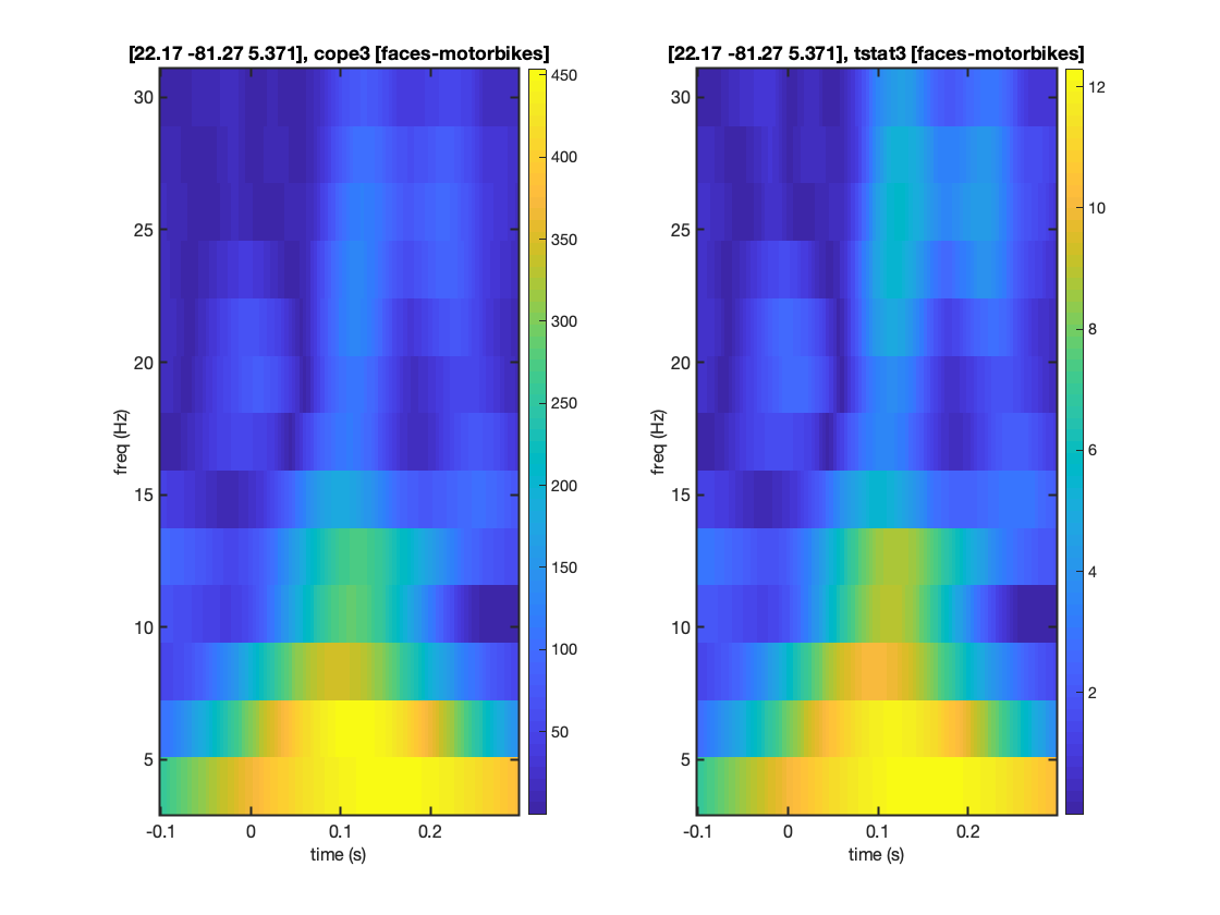
As with the other analyses, take a look at the first level summary report. Alongside the first level design matrix, this contains the COPE and t-stat estimates across the whole time-frequency decomposition from the peak ROI. The results are uniform within each parcel in the whole brain orthoplots and indicate the largest responses around 116ms after stimulus onset are in visual cortex for all three contrasts.

disp(oat.results.report.html_fname);

/Users/andrew/toolboxes/osl/example_data/faces_subject1_data_osl2/beamformer_erf.oat/plots/report.html

SOURCE ROI TIME-FREQUENCY PLOT

As with the voxel example able, we can interrogate the OAT to extract the time-frequency plots from specific contrasts.

This time the results come from the parcel containing the requested voxel.

mni_coord=[4,-82,-8]; % Visual Cortex Voxel

S2=[];
S2.vox_coord=mni_coord;
S2.stats=oat.first_level.results_fnames{1};
S2.oat=oat;
S2.first_level_cons_to_do = [3]; % plots all of these contrasts

[vox_ind_used] = oat_plot_vox_stats(S2);

SOURCE ROI SINGLE-FREQUENCY POWER PLOT

We may also isolate the results from a single frequency by defining the freq_inds parameter. The code below will plot the OAT results over time for the 8Hz frequency band.

Note that first two contrasts in the GLM are testing whether the power at a given time and frequency is different from zero. As such the COPE and t-stats return high values, even within the pre-stimulus period. This reflects the fact that there is always some power at 8Hz, though the later time-points clearly indicate that this power is modulated by stimulus onset.

The faces-motorbikes contrast is looking for differences in power. This quantity is not strictly positive so we do see t-values around zero in the prestimulus period.

Taken together, these results indicate that there is none-zero power at 8Hz through the epoch, though it is modulated by stimulus onset, moreover faces show a greater modulation of power than motorbikes.

% Load first level results
stats=oat_load_results(oat,oat.first_level.results_fnames{1});

% Define frequency of interest
freqbin=nearest(stats.frequencies,8); % find bin for 8Hz

% Define location of interest
mni_coord=[4,-82,-8]; % Visual Cortex Voxel

S2=[];
S2.vox_coord=mni_coord;
S2.stats=stats;
S2.oat=oat;
S2.freq_inds=freqbin;
S2.first_level_cons_to_do=[2,1,3]; % plots all of these contrasts
[vox_ind_used] = oat_plot_vox_stats(S2);

Published with MATLAB® R2019a