OAT 2 - Sensorspace Time-Frequency Analysis

In this practical we will work with a single subject's data from an emotional faces task (data courtesy of Susie Murphy) and perform an Time-Frequency analysis in sensor space.

Please read each cell in turn before copying its contents either directly into the MatLab console or your own blank script. By the end of this session you should have created your own template analysis script which can be applied to further analysis.

You will need the following files from the example_data directory:

Contents

INITIALISE GLOBAL SETTINGS FOR THIS ANALYSIS

This cell sets the directory that OAT will work in. Change the workingdir variable to correspond to the correct directory on your computer before running the cell.

% directory where the data is:
datadir = fullfile(osldir,'example_data','faces_singlesubject','spm_files');

% directory to put the analysis in
workingdir = fullfile(osldir,'example_data','faces_singlesubject');

SET UP THE SUBJECTS FOR THE ANALYSIS

Specify a list of the SPM input files. Note that here we only have 1 subject, but more generally there would be more than one. For example:

spm_files_continuous{1} = [workingdir '/sub1_face_sss.mat'];

spm_files_continuous{2} = [workingdir '/sub2_face_sss.mat'];

etc...

% clear old spm files
clear spm_files_continuous spm_files_epoched

spm_files_continuous{1}=fullfile(datadir,'Aface_meg1.mat');
spm_files_epoched{1}=fullfile(datadir,'eAface_meg1.mat');

SETUP SENSOR SPACE SOURCE RECON

This stage sets up the source reconstruction stage of an OAT analysis. The source_recon stage is always run even for a sensor space analysis, though in these cases it simply prepares the data for the subsequent OAT stages.

In this example we define our input files (D_continuous and D_epoched) and conditions before setting a time frequency window from -200ms before stimulus onset, to 400ms after and from 4Hz to 100Hz. The source recon method is set to 'none' as we are performing a sensorspace analysis. The oat.source_recon.dirname is where all the analysis results will be stored. This includes all the intermediate steps, diagnostic plots and final results.

oat=[];
oat.source_recon.D_epoched=spm_files_epoched; % this is passed in so that the bad trials and bad channels can be read out
oat.source_recon.D_continuous=spm_files_continuous;
oat.source_recon.conditions={'Motorbike','Neutral face','Happy face','Fearful face'};
oat.source_recon.freq_range=[4 100]; % frequency range in Hz
oat.source_recon.time_range=[-0.2 0.4];
oat.source_recon.method='none';
oat.source_recon.normalise_method='none';

% Set this to something specific, this the directory where the OAT will be
% stored
oat.source_recon.dirname = fullfile(workingdir,'sensorspace_tf');

SETUP THE TIME-FREQUENCY DECOMPOSITION

Next we set up a single subject trial-wise GLM on our prepared data. Firstly the time-frequency parameters are defined, these must be within the bounds of the time-frequency window set in the source recon stage.

Note the following settings in particular:

Note that you can also do time-frequency analyses outside of OAT by passing an SPM MEEG object straight into the osl_tf_transform function.

We have also set the baseline correction to be turned off for the third contrast, [-3 1 1 1] (this is often a good idea for differential contrasts, for which we do not need to do baseline correction):

oat.first_level.tf_method='morlet'; % can be morlet or hilbert
oat.first_level.tf_freq_range=[5 40]; % frequency range in Hz
oat.first_level.time_range=[-0.2 0.3]; % need to make this time range smallet than oat.source_recon.time_range to remove edge effects
oat.first_level.tf_num_freqs=14; % we are keeping this unusally low in the practical for the sake of speed
%oat.first_level.tf_hilbert_freq_res=8;

% NOTE that you can also set HILBERT freq ranges explicitly, e.g.:
% |oat.first_level.tf_hilbert_freq_ranges=[[4 8];[8 12];[12 16];[16 20];[20 24];[24 30]];| % frequency range in Hz

oat.first_level.post_tf_downsample_factor=4; % does downsampling after the TF decomposition

oat.first_level.bc=[1 1 0]; % specifies whether or not baseline correction is done for the different contrasts

SETUP THE FIRST LEVEL GLM

This cell defines the GLM parameters for the first level analysis. Critically this includes the design matrix (in Xsummary) and the contrast matrix. Xsummary is a parsimonious description of the design matrix. It contains values Xsummary{reg,cond}, where reg is a regressor index number and cond indexes different experimental conditions (e.g. pictures of faces, pictures of motorbikes). This will be used (by expanding the conditions over trials) to create the (num_regressors x num_trials) design matrix.

Each contrast is a vector containing a weight per condition defining how the condition parameter estimates are to be compared. Each vector will produce a different t-map across the sensors. Contrasts 1 and 2 describe positive correlations between each sensor's activity and the presence of a motorbike or face stimulus respectively. Contrast 3 tests whether each sensor's activity is larger for faces than motorbikes.

Xsummary={};
Xsummary{1}=[1 0 0 0];
Xsummary{2}=[0 1 0 0];
Xsummary{3}=[0 0 1 0];
Xsummary{4}=[0 0 0 1];
oat.first_level.design_matrix_summary=Xsummary;

% contrasts to be calculated:
oat.first_level.contrast={};
oat.first_level.contrast{1}=[3 0 0 0]'; % motorbikes
oat.first_level.contrast{2}=[0 1 1 1]'; % faces
oat.first_level.contrast{3}=[-3 1 1 1]'; % faces-motorbikes
oat.first_level.contrast_name{1}='motorbikes';
oat.first_level.contrast_name{2}='faces';
oat.first_level.contrast_name{3}='faces-motorbikes';

oat.first_level.cope_type='cope';
oat.first_level.report.first_level_cons_to_do=[2 1 3];
oat.first_level.report.modality_to_do='MEGPLANAR';
oat.first_level.bc=[0 0 0];

RUN OAT

We now run the source-recon and first-level OAT stages

OAT will produce and close a number of figures as it processes, we will discuss what they mean once it has finished (this takes a couple of minutes)

oat.to_do=[1 1 0 0];
oat = osl_run_oat(oat);

Detected Elekta Neuromag 306 data. Using default Elekta Neuromag 306 settings.
Warning: oat.source_recon.modalities not set, or not set properly. Will set to
default:MEGPLANARMEGMAG 
oat.source_recon.D_epoched set. OAT will do an epoched data trial-wise GLM
*************************************************************
Running source_recon
*************************************************************
%%%%%%%%%%%%%%%%%%%%%%%%%%%%%%%%%%%%%%%%%%%%%%%%%%%%%%%%%%%%%%%%%%%%%%%%%%%%%%%%%%%%%%%%%%%%%%
%%%%%%%%%%%%%%%%%%%%%%%  RUNNING OAT SOURCE RECON (SENSOR SPACE SETUP) ON SESS = 1  %%%%%%%%%%%%%%%%%%%%%%%
Using continuous data as input
Using epoched data as input
Preparing source recon stage for /Users/andrew/toolboxes/osl/example_data/faces_singlesubject/spm_files/Aface_meg1.mat
Will be designated session1

SPM12: spm_eeg_copy (v7132)                        01:46:08 - 11/11/2019
========================================================================

SPM12: spm_eeg_copy (v7132)                        01:46:11 - 11/11/2019
========================================================================
Temporal filtering...

SPM12: spm_eeg_filter (v7125)                      01:46:14 - 11/11/2019
========================================================================
Filter bandpass (but, twopass)          :                    [4  100] Hz
Completed                               :          01:46:26 - 11/11/2019
Epoching...
Doing no within-trial baseline correction at the point of epoching

SPM12: spm_eeg_epochs (v7125)                      01:46:26 - 11/11/2019
========================================================================
Data type is missing or incorrect, assigning default.
Baseline correction                     :                              0
Number of trials                        :                            360
Completed                               :          01:46:38 - 11/11/2019
Changing the number of channels, so discarding online montages.

SPM12: spm_eeg_copy (v7132)                        01:46:49 - 11/11/2019
========================================================================
Saving source recon (sensorspace setup) results: session1_recon
*************************************************************
Running first_level
*************************************************************
%%%%%%%%%%%%%%%%%%%%%%%%%%%%%%%%%%%%%%%%%%%%%%%%%%%%%%%%%%%%%%%%%%%%%%%%%%%%%%%%%%%%%%%%%%%%%%
%%%%%%%%%%%%%%%%%%%%%%%  RUNNING OAT FIRST LEVEL ON SESS = 1  %%%%%%%%%%%%%%%%%%%%%%%

ans =

    '/Users/andrew/toolboxes/osl/example_data/faces_singlesubject/sensorspace_tf.oat/efsession1_spm_meeg.mat'


SPM12: spm_eeg_copy (v7132)                        01:47:00 - 11/11/2019
========================================================================

ans =

    '/Users/andrew/toolboxes/osl/example_data/faces_singlesubject/sensorspace_tf.oat/efsession1_spm_meeg_firstlevel.mat'

Working in sensor space
Creating Morlet basis set.  If you are seeing message many times, you may wish to pass a morlet basis set to 'osl_tf_transform'
USING MORLET TF
Freqs: 5      7.69231      10.3846      13.0769      15.7692      18.4615      21.1538      23.8462      26.5385      29.2308      31.9231      34.6154      37.3077           40
Reconstruct time courses and computing stats for dataset session1_recon
CAREFUL: are you sure you want no first_level.do_glm_demean flag on with no constant regressors in the design matrix!!!!?
State 1 is active for 213.6secs
First level COPEs outputted will have dimension Nvoxels x Ntpts x Ncontrasts x Nfreqs:
306   31    3   14
Doing T-F transform in sensor space on [3.65384615384615 6.34615384615385] Hz...
size(sens_data_tf)=[325 38 356 1], (nsens x ntpts x ntri x nfreq)
Doing Morlet transform...
100.00 %
 - estimated time to finish is 0 seconds
Doing T-F transform in sensor space on [6.34615384615385 9.03846153846154] Hz...
size(sens_data_tf)=[325 38 356 1], (nsens x ntpts x ntri x nfreq)
Doing Morlet transform...
100.00 %
 - estimated time to finish is 0 seconds
Doing T-F transform in sensor space on [9.03846153846154 11.7307692307692] Hz...
size(sens_data_tf)=[325 38 356 1], (nsens x ntpts x ntri x nfreq)
Doing Morlet transform...
100.00 %
 - estimated time to finish is 0 seconds
Doing T-F transform in sensor space on [11.7307692307692 14.4230769230769] Hz...
size(sens_data_tf)=[325 38 356 1], (nsens x ntpts x ntri x nfreq)
Doing Morlet transform...
100.00 %
 - estimated time to finish is 0 seconds
Doing T-F transform in sensor space on [14.4230769230769 17.1153846153846] Hz...
size(sens_data_tf)=[325 38 356 1], (nsens x ntpts x ntri x nfreq)
Doing Morlet transform...
100.00 %
 - estimated time to finish is 0 seconds
Doing T-F transform in sensor space on [17.1153846153846 19.8076923076923] Hz...
size(sens_data_tf)=[325 38 356 1], (nsens x ntpts x ntri x nfreq)
Doing Morlet transform...
100.00 %
 - estimated time to finish is 0 seconds
Doing T-F transform in sensor space on [19.8076923076923 22.5] Hz...
size(sens_data_tf)=[325 38 356 1], (nsens x ntpts x ntri x nfreq)
Doing Morlet transform...
100.00 %
 - estimated time to finish is 0 seconds
Doing T-F transform in sensor space on [22.5 25.1923076923077] Hz...
size(sens_data_tf)=[325 38 356 1], (nsens x ntpts x ntri x nfreq)
Doing Morlet transform...
100.00 %
 - estimated time to finish is 0 seconds
Doing T-F transform in sensor space on [25.1923076923077 27.8846153846154] Hz...
size(sens_data_tf)=[325 38 356 1], (nsens x ntpts x ntri x nfreq)
Doing Morlet transform...
100.00 %
 - estimated time to finish is 0 seconds
Doing T-F transform in sensor space on [27.8846153846154 30.5769230769231] Hz...
size(sens_data_tf)=[325 38 356 1], (nsens x ntpts x ntri x nfreq)
Doing Morlet transform...
100.00 %
 - estimated time to finish is 0 seconds
Doing T-F transform in sensor space on [30.5769230769231 33.2692307692308] Hz...
size(sens_data_tf)=[325 38 356 1], (nsens x ntpts x ntri x nfreq)
Doing Morlet transform...
100.00 %
 - estimated time to finish is 0 seconds
Doing T-F transform in sensor space on [33.2692307692308 35.9615384615385] Hz...
size(sens_data_tf)=[325 38 356 1], (nsens x ntpts x ntri x nfreq)
Doing Morlet transform...
100.00 %
 - estimated time to finish is 0 seconds
Doing T-F transform in sensor space on [35.9615384615385 38.6538461538462] Hz...
size(sens_data_tf)=[325 38 356 1], (nsens x ntpts x ntri x nfreq)
Doing Morlet transform...
100.00 %
 - estimated time to finish is 0 seconds
Doing T-F transform in sensor space on [38.6538461538462 41.3461538461538] Hz...
size(sens_data_tf)=[325 38 356 1], (nsens x ntpts x ntri x nfreq)
Doing Morlet transform...
100.00 %
 - estimated time to finish is 0 seconds
reading layout from file /Users/andrew/toolboxes/osl/layouts/neuromag306planar3.lay
the call to "ft_prepare_layout" took 0 seconds and required the additional allocation of an estimated NaN MB
reading layout from file /Users/andrew/toolboxes/osl/layouts/neuromag306planar2.lay
the call to "ft_prepare_layout" took 0 seconds and required the additional allocation of an estimated NaN MB
reading layout from file /Users/andrew/toolboxes/osl/layouts/neuromag306mag.lay
the call to "ft_prepare_layout" took 0 seconds and required the additional allocation of an estimated NaN MB
reading layout from file /Users/andrew/toolboxes/osl/layouts/neuromag306cmb.lay
the call to "ft_prepare_layout" took 0 seconds and required the additional allocation of an estimated NaN MB
Averaging the (A)COPEs for orthogonal planar gradiometers
Changing the number of channels, so discarding online montages.
Changing the number of channels, so discarding online montages.
Saving statistics in file /Users/andrew/toolboxes/osl/example_data/faces_singlesubject/sensorspace_tf.oat/session1_first_level
Changing the number of channels, so discarding online montages.
Changing the number of channels, so discarding online montages.
the call to "ft_selectdata" took 0 seconds and required the additional allocation of an estimated NaN MB
reading layout from file /Users/andrew/toolboxes/osl/layouts/neuromag306cmb.lay
the call to "ft_prepare_layout" took 0 seconds and required the additional allocation of an estimated NaN MB
the call to "ft_multiplotTFR" took 1 seconds and required the additional allocation of an estimated NaN MB
reading layout from file /Users/andrew/toolboxes/osl/layouts/neuromag306cmb.lay
the call to "ft_prepare_layout" took 0 seconds and required the additional allocation of an estimated NaN MB
the call to "ft_selectdata" took 0 seconds and required the additional allocation of an estimated NaN MB
the call to "ft_topoplotTFR" took 1 seconds and required the additional allocation of an estimated NaN MB
Changing the number of channels, so discarding online montages.
Changing the number of channels, so discarding online montages.
the call to "ft_selectdata" took 0 seconds and required the additional allocation of an estimated NaN MB
reading layout from file /Users/andrew/toolboxes/osl/layouts/neuromag306cmb.lay
the call to "ft_prepare_layout" took 0 seconds and required the additional allocation of an estimated NaN MB
the call to "ft_multiplotTFR" took 1 seconds and required the additional allocation of an estimated NaN MB
reading layout from file /Users/andrew/toolboxes/osl/layouts/neuromag306cmb.lay
the call to "ft_prepare_layout" took 0 seconds and required the additional allocation of an estimated NaN MB
the call to "ft_selectdata" took 0 seconds and required the additional allocation of an estimated NaN MB
the call to "ft_topoplotTFR" took 1 seconds and required the additional allocation of an estimated NaN MB
Changing the number of channels, so discarding online montages.
Changing the number of channels, so discarding online montages.
the call to "ft_selectdata" took 0 seconds and required the additional allocation of an estimated NaN MB
reading layout from file /Users/andrew/toolboxes/osl/layouts/neuromag306cmb.lay
the call to "ft_prepare_layout" took 0 seconds and required the additional allocation of an estimated NaN MB
the call to "ft_multiplotTFR" took 1 seconds and required the additional allocation of an estimated NaN MB
reading layout from file /Users/andrew/toolboxes/osl/layouts/neuromag306cmb.lay
the call to "ft_prepare_layout" took 0 seconds and required the additional allocation of an estimated NaN MB
the call to "ft_selectdata" took 0 seconds and required the additional allocation of an estimated NaN MB
the call to "ft_topoplotTFR" took 0 seconds and required the additional allocation of an estimated NaN MB
View first level report at:
/Users/andrew/toolboxes/osl/example_data/faces_singlesubject/sensorspace_tf.oat/plots/first_level/sess_session1_MEGPLANAR/report.html
To view OAT report, point your browser to <a href="/Users/andrew/toolboxes/osl/example_data/faces_singlesubject/sensorspace_tf.oat/plots/report.html">/Users/andrew/toolboxes/osl/example_data/faces_singlesubject/sensorspace_tf.oat/plots/report.html</a>

READ REPORT

OAT runs the GLM for every time point and frequency band across all sensors.

OAT will create a report containing a summary of the first level analysis results (as well as some diagnostic figures from the source reconstruction). The specific content of this report depends upon settings in oat.first_level.report:

Open the report indicated in oat.results.report in a web browser (there will also be a link to this available in the Matlab output). This displays the diagnostic plots.

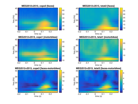
This brings up a list of sessions. Here we have only preprocessed one session. Click on the "Session 1 report" link to bring up the diagnostic plots for session 1 and take a look.

The settings in the current OAT will generate an image with the COPE and t-stats for all three contrasts from the sensor with the maximum statistic for contrast 2 (faces) from the planar gradiometers as seen below

disp(oat.results.report.html_fname); % show path to web page report

/Users/andrew/toolboxes/osl/example_data/faces_singlesubject/sensorspace_tf.oat/plots/report.html

GENERATE ALTERNATIVE REPORT OF TIME-FREQUENCY RESULTS

The oat_first_level_stats_report function can be used to produce alternative OAT reports using an already run OAT.

Here, we will create a new report where we have changed the report to view the results from the magnetometers (the default report showed results from MEGPLANAR), and to only show the motorbikes vs. faces contrast (contrast 3).

% Report settings
oat.first_level.report.modality_to_do='MEGMAG';
oat.first_level.report.first_level_cons_to_do=[3];

% Regenerate report
report = oat_first_level_stats_report(oat,oat.first_level.results_fnames{1});

% Open the report in matlabs html browser
open(report.html_fname);

Changing the number of channels, so discarding online montages.
Changing the number of channels, so discarding online montages.
the call to "ft_selectdata" took 0 seconds and required the additional allocation of an estimated NaN MB
reading layout from file /Users/andrew/toolboxes/osl/layouts/neuromag306mag.lay
the call to "ft_prepare_layout" took 0 seconds and required the additional allocation of an estimated NaN MB
the call to "ft_multiplotTFR" took 2 seconds and required the additional allocation of an estimated NaN MB
reading layout from file /Users/andrew/toolboxes/osl/layouts/neuromag306mag.lay
the call to "ft_prepare_layout" took 0 seconds and required the additional allocation of an estimated NaN MB
the call to "ft_selectdata" took 0 seconds and required the additional allocation of an estimated NaN MB
the call to "ft_topoplotTFR" took 0 seconds and required the additional allocation of an estimated NaN MB
View first level report at:
/Users/andrew/toolboxes/osl/example_data/faces_singlesubject/sensorspace_tf.oat/plots/first_level/sess_session1_MEGMAG/report.html

RESULTS

The results are stored in the oat structure and the can be loaded back into matlab using oat_load_results.

This is useful for checking over results of the GLM or as the basis for further analyses.

disp('oat.results:');
disp(oat.results);

% load first-level GLM result
stats1=oat_load_results(oat,oat.first_level.results_fnames{1});

oat.results:
        date: '11-Nov-2019'
    plotsdir: '/Users/andrew/toolboxes/osl/example_data/faces_singlesubject/sensorspace_tf.oat/plots'
     logfile: '/Users/andrew/toolboxes/osl/example_data/faces_singlesubject/sensorspace_tf.oat/plots/log-11-Nov-2019.txt'
      report: [1×1 struct]

VISUALISE USING FIELDTRIP

A lot of the visualisations work using functions from fieldtrip. These offer a wide range of visualisation options and are high customisable. Here we will use an OSL function which plots an OAT result in a fieldtrip multiplot.

We will plot the T-stat time-frequency results for the faces contrast across all the Planar Gradiometers by defining the following options and calling oat_stats_multiplotTFR.

Note that this produces an interactive figure, with which you can:

S2=[];
S2.oat=oat;
S2.stats_fname=oat.first_level.results_fnames{1};
S2.modality='MEGPLANAR';
S2.first_level_contrast=[2];
S2.cfg.colorbar='yes';
S2.cfg.zlim = [0 35];
S2.view_cope=0;

% calculate t-stat using contrast of absolute value of parameter estimates
[cfg, data]=osl_stats_multiplotTFR(S2);
title([oat.first_level.contrast_name{S2.first_level_contrast}]);

Changing the number of channels, so discarding online montages.
Changing the number of channels, so discarding online montages.
the call to "ft_selectdata" took 0 seconds and required the additional allocation of an estimated NaN MB
reading layout from file /Users/andrew/toolboxes/osl/layouts/neuromag306cmb.lay
the call to "ft_prepare_layout" took 0 seconds and required the additional allocation of an estimated NaN MB
the call to "ft_multiplotTFR" took 2 seconds and required the additional allocation of an estimated NaN MB

CREATE A TOPOPLOT AVERAGED WITHIN A TF WINDOW

We often want to focus our visualisations on specific points in time or frequency rather than looking at the everything at once.

The following code calls creates a topoplot from the same results as the previous section, but now averages the results over 130 to 160 ms, and 8 to 12 Hz.

cfg.xlim        = [0.13 0.16]; % time window in secs
cfg.ylim        = [8 12]; % freq window in Hz
cfg.interactive = 'no';
figure; ft_topoplotTFR(cfg,data);
title([oat.first_level.contrast_name{S2.first_level_contrast}]);

reading layout from file /Users/andrew/toolboxes/osl/layouts/neuromag306cmb.lay
the call to "ft_prepare_layout" took 0 seconds and required the additional allocation of an estimated NaN MB
the call to "ft_selectdata" took 0 seconds and required the additional allocation of an estimated NaN MB
the call to "ft_topoplotTFR" took 0 seconds and required the additional allocation of an estimated NaN MB

Published with MATLAB® R2019a