Data structures - MEEG and NIFTI
There are a handful of useful data structures provided by SPM and OSL to facilitate working with MEG data. Becoming comfortable with these data structures will help when working with OSL. This example gives a (very brief) overview of the two most important containers for MEG data and for MRI data used in OSL.
Contents
SPM MEEG objects
First up is the MEEG object. This is a container for the actual MEG data itself. These live on disk in two files
- a .dat file, which contains the time series data
- a .mat that contains header information
You can load this object into Matlab using spm_eeg_load:
D = spm_eeg_load(fullfile(osldir,'example_data','roinets_example','subject_1'))
SPM M/EEG data object
Type: continuous
Transform: time
1 conditions
276 channels
11251 samples/trial
1 trials
Sampling frequency: 250 Hz
Loaded from file  /Users/romesh/oxford_postdoc/toolboxes/osl/example_data/roinets_example/subject_1.mat

2 online montage(s) setup
Current montage applied (0=none): 0

Use the syntax D(channels, samples, trials) to access the data
Type "methods('meeg')" for the list of methods performing other operations with the object
Type "help meeg/method_name" to get help about methods
You can access the data by indexing this object
x = D(:,:,:);
size(x)
ans =

         276       11251
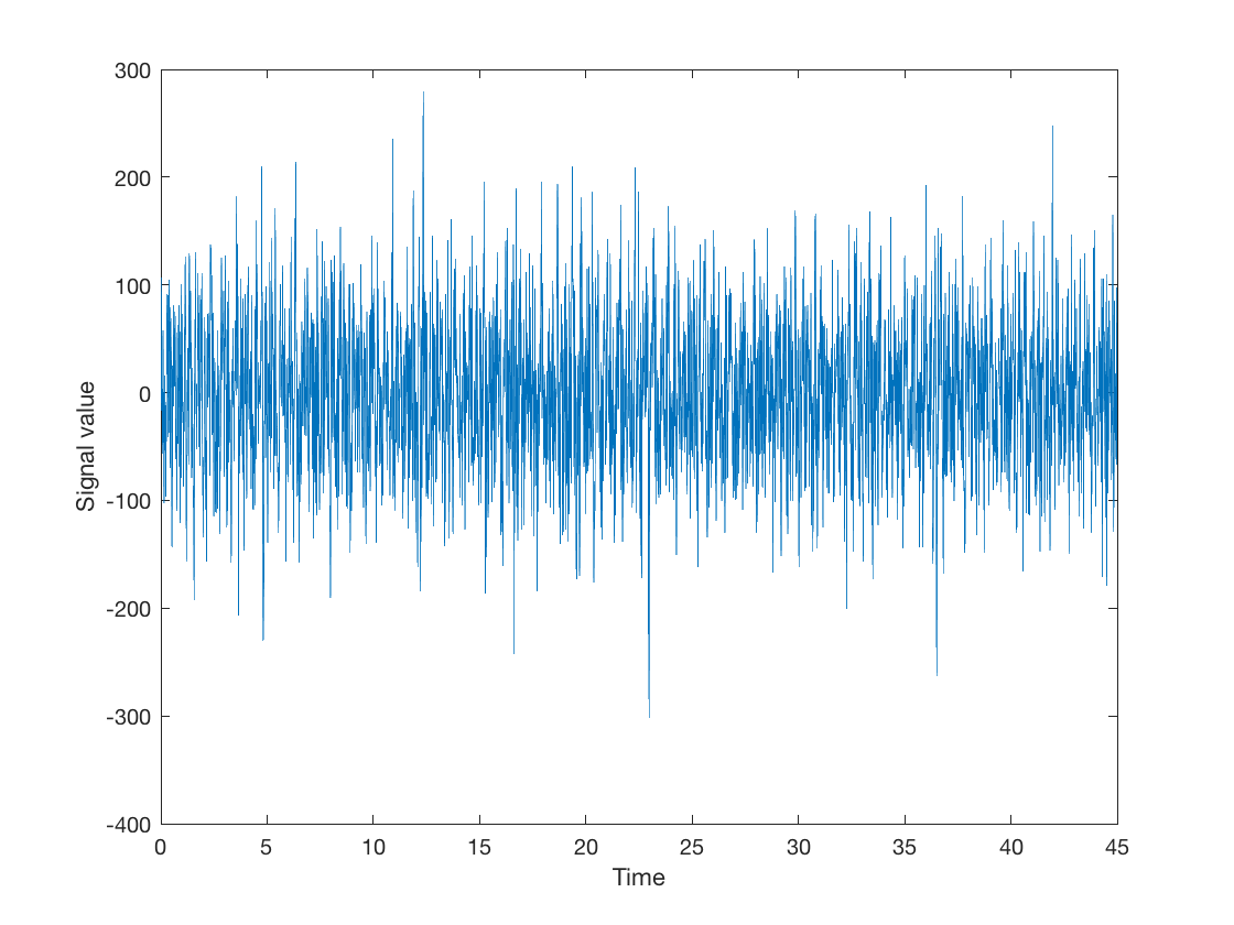
For continuous data, this matrix will be channels x time. For epoched data, there is an additional dimension corresponding to trial. You can access the time points easily as well, and use this to quickly plot your data
t = D.time;
plot(t,x(3,:))
xlabel('Time')
ylabel('Signal value')
How do you know what signal you are plotting? You can get information from the header about the channels
D.chanlabels(3) % channel name
D.chantype(3) % type of sensor
D.units(3) % data units
ans =

  cell

    'MLC11'


ans =

  cell

    'MEGGRAD'


ans =

  cell

    'fT'
and there are other useful properties about the data in the MEEG object
D.fsample % Sampling rate
D.nchannels % Number of channels
D.fname % Name of the mat file
ans =

   250


ans =

   276


ans =

    'subject_1.mat'
If you make changes to the MEEG object, these can be saved to disk using
D.save();
To copy the file, use
D2 = D.copy('./test');
This is one potentially confusing part of MEEG objects - most of their methods return new MEEG objects. So for example
D.fname
D2.fname
ans =

    'subject_1.mat'


ans =

    'test.mat'
Now we will experiment with changing information in the header
clear D D2
D = spm_eeg_load('test.mat')
SPM M/EEG data object
Type: continuous
Transform: time
1 conditions
276 channels
11251 samples/trial
1 trials
Sampling frequency: 250 Hz
Loaded from file  /Users/romesh/oxford_postdoc/toolboxes/osl/std_masks/test.mat

2 online montage(s) setup
Current montage applied (0=none): 0

Use the syntax D(channels, samples, trials) to access the data
Type "methods('meeg')" for the list of methods performing other operations with the object
Type "help meeg/method_name" to get help about methods
We have loaded the new copy so that we don't accidentally make changes to the original data. Most properties of MEEG objects need to be set through their methods. For example, we can set the sampling rate using
D.fsample(200)
SPM M/EEG data object
Type: continuous
Transform: time
1 conditions
276 channels
11251 samples/trial
1 trials
Sampling frequency: 200 Hz
Loaded from file  /Users/romesh/oxford_postdoc/toolboxes/osl/std_masks/test.mat

2 online montage(s) setup
Current montage applied (0=none): 0

Use the syntax D(channels, samples, trials) to access the data
Type "methods('meeg')" for the list of methods performing other operations with the object
Type "help meeg/method_name" to get help about methods
But there is a catch!
D.fsample
ans =

   250
As you can see, D.fsample(200) returns a new MEEG object, without changing the old object. So we need to do
D = D.fsample(200);
D.fsample
ans =

   200
This change is not automatically saved to disk. For example
D = spm_eeg_load('test.mat');
D.fsample
ans =

   250
We need to save the updated header to disk manually
D = D.fsample(200);
D.save()
D = spm_eeg_load('test.mat');
D.fsample
SPM M/EEG data object
Type: continuous
Transform: time
1 conditions
276 channels
11251 samples/trial
1 trials
Sampling frequency: 200 Hz
Loaded from file  /Users/romesh/oxford_postdoc/toolboxes/osl/std_masks/test.mat

2 online montage(s) setup
Current montage applied (0=none): 0

Use the syntax D(channels, samples, trials) to access the data
Type "methods('meeg')" for the list of methods performing other operations with the object
Type "help meeg/method_name" to get help about methods


ans =

   200
This changes the contents of the '.mat' file but not the '.dat' file, because the raw data itself hasn't changed. One extremely important thing to understand about MEEG objects is that they memory-map the .dat file. This means when you run D(1,:,:) you are indexing into the .dat file directly. While changing the header requires saving the MEEG object, any changes you make to the raw data occur on disk immediately. So for example
D(1,1)
D(1,1) = 0
ans =

    0.7085

SPM M/EEG data object
Type: continuous
Transform: time
1 conditions
276 channels
11251 samples/trial
1 trials
Sampling frequency: 200 Hz
Loaded from file  /Users/romesh/oxford_postdoc/toolboxes/osl/std_masks/test.mat

2 online montage(s) setup
Current montage applied (0=none): 0

Use the syntax D(channels, samples, trials) to access the data
Type "methods('meeg')" for the list of methods performing other operations with the object
Type "help meeg/method_name" to get help about methods
This immediately writes a value of 0 to disk. So if we reload the MEEG object:
D = spm_eeg_load('test.mat');
D(1,1)
ans =

     0
You can see the change persists even though '.save()' was never called. This is the main reason why some OSL operations return a MEEG object without making changes on disk (because they change the header, which is only written when 'save()' is called) while others make copies of the MEEG object (e.g. filtering results in a new file with a prefix of 'f' because otherwise the original data would be instantly overwritten). It's important to keep this in mind, because if you happen to run
D(:,:,:) = 0
SPM M/EEG data object
Type: continuous
Transform: time
1 conditions
276 channels
11251 samples/trial
1 trials
Sampling frequency: 200 Hz
Loaded from file  /Users/romesh/oxford_postdoc/toolboxes/osl/std_masks/test.mat

2 online montage(s) setup
Current montage applied (0=none): 0

Use the syntax D(channels, samples, trials) to access the data
Type "methods('meeg')" for the list of methods performing other operations with the object
Type "help meeg/method_name" to get help about methods
your data is now gone, and you would need to restore it from a separate backup (which you presumably made before starting!). In our case, we can just reload the original file (before we copied it) - and make a new copy, just to be safe!
D = spm_eeg_load(fullfile(osldir,'example_data','roinets_example','subject_1'))
D.copy('./test');
SPM M/EEG data object
Type: continuous
Transform: time
1 conditions
276 channels
11251 samples/trial
1 trials
Sampling frequency: 250 Hz
Loaded from file  /Users/romesh/oxford_postdoc/toolboxes/osl/example_data/roinets_example/subject_1.mat

2 online montage(s) setup
Current montage applied (0=none): 0

Use the syntax D(channels, samples, trials) to access the data
Type "methods('meeg')" for the list of methods performing other operations with the object
Type "help meeg/method_name" to get help about methods
The final important aspect of MEEG objects is the 'online montage'. An online montage is a linear combination of the original sensor data. This can be used to represent any linear operation, including ICA artefact rejection, beamforming, parcellation, and leakage correction. Writing these combinations as linear transformations rather than actual data enables a considerable saving of disk space. You can list the montages present using has_montage
has_montage(D)
*0 - none (276 channels)
1 - without weights normalisation, class 1 (3559 channels)
2 - with weights normalisation, class 1 (3559 channels)
To switch montages, you can use
D.nchannels
D = D.montage('switch',2);
D.nchannels
ans =

   276


ans =

        3559
Montage 0 corresponds to the raw sensor data. You can also get information about the montage, including the linear transformation matrix
D.montage('getmontage',2)
ans =

  struct with fields:

        name: 'with weights normalisation, class 1'
         tra: [3559×276 double]
    labelnew: {3559×1 cell}
    labelorg: {276×1 cell}
    channels: [1×3559 struct]
To add an online montage of your own, use the add_montage function. For example, if we have a single channel that we want to correspond to the sum of all of the sensors, we could use
D = D.montage('switch',0);
tmp = sum(D(:,1)) % The target value at the first timepoint
D = add_montage(D,ones(1,D.nchannels),'My new montage');
has_montage(D)
D(1,1)
tmp =

   1.5465e+03

No new channels information : setting channels info automatically.
0 - none (276 channels)
1 - without weights normalisation, class 1 (3559 channels)
2 - with weights normalisation, class 1 (3559 channels)
*3 - My new montage (1 channels)

ans =

   1.5465e+03
Note that because the montage information is stored in the header, the save() method must be used to save changes that affect montages e.g.
D = spm_eeg_load(fullfile(osldir,'example_data','roinets_example','subject_1'));
has_montage(D)
*0 - none (276 channels)
1 - without weights normalisation, class 1 (3559 channels)
2 - with weights normalisation, class 1 (3559 channels)
NIFTI files
NIFTI files are typically used to store volumetric image data, for example, structural scans. Fundamentally they are simply a means of storing a multidimensional matrix in a binary file. They come in two varieties
- .nii which is the file itself
- .nii.gz which is a gzipped version of the .nii file.
Most programs designed to work with NIFTI files will accept either kind of file. Here are some NIFTI files that are supplied with OSL
standard_brain = fullfile(osldir,'std_masks','MNI152_T1_1mm_brain.nii.gz');
standard_4mm_brain = fullfile(osldir,'std_masks','MNI152_T1_4mm_brain.nii.gz');
ft_4mm_brain = fullfile(osldir,'std_masks','ft_4mm_brain.nii.gz');
The first is a standard brain image, the second is a weighted parcellation. You can load the data in these files into MATLAB using
vol = nii.load(standard_brain);
size(vol)
ans =

   182   218   182
If you have previously used OSL, note that nii.load is equivalent to read_avw except it does not require FSL. When you use nii.load, the contents of the NIFTI file are loaded in as a matrix. However, what is the spatial location of this data? Additional information is required to compute which part of space the matrix occupies. You can do this with the xform matrix in the header of the NIFTI file. This matrix describes the coordinate system in which to interpret the matrix, as well as accounting for any transformations (e.g. deformations) that should be applied to the data. This matrix is also read in by nii.load
[vol,res,xform] = nii.load(standard_brain);
res
xform
res =

     1     1     1     1


xform =

    -1     0     0    90
     0     1     0  -126
     0     0     1   -72
     0     0     0     1
To save a NIFTI file, you can use nii.save().
nii.save(vol,res,xform,'newfile.nii.gz');
Make sure that you include the extension (.nii or .nii.gz) when saving the file. You can optionally leave res and xform blank when saving the file. However, be aware that xform is considered critical information, and omitting it can make your data unusable. In particular, some NIFTI files are saved with the X-axis reversed. This information is stored in the xform matrix. Notice how these two files have different signs in the top-left entry
[~,~,xform] = nii.load(standard_4mm_brain)
[~,~,xform] = nii.load(ft_4mm_brain)
xform =

    -4     0     0    90
     0     4     0  -126
     0     0     4   -72
     0     0     0     1


xform =

     4     0     0   -74
     0     4     0  -112
     0     0     4   -72
     0     0     0     1
NIFTI viewers such as fsleyes and osleyes will use the information in xform to appropriately orient the image so that it is displayed correctly on screen. Without this information, left and right can easily become reversed accidentally! If you try to load in a NIFTI file that might not have this information saved properly, nii.load will display a warning. This warning will also be displayed if your data is in a different coordinate system to standard MNI space. For example, if you have a raw structural scan, its coordinate system will probably correspond to the scanner space, rather than brain space. It is difficult to reliably superimpose images in different coordinate systems.