Coregistration with SPM and RHINO

This tutorial covers the registration of MRI and M/EEG datasets into a common space to allow for analysis in sourcespace.

This practical uses data from the coreg_example subfolders in the OSL example_data directory. Please make sure this is present before starting.

Contents

Coordinate Systems

There are several co-ordinate systems which must be aligned before we can project our sensor MEG data into source space. These are:

See https://ohba-analysis.github.io/osl-docs/pages/docs/preprocessing.html#coregistration-using-rhino for more information.

Coregistration summary

The coregistration follows these steps

Once these transforms have been identified we can move between MEG sensors and specific locations within the MRI scan.

Setup the analysis

To start OSL only thing you need to do is to go into your OSL directory (i.e. type cd /somedirectory/osl-core ) and then run the following.

osl_startup;

This only needs to be run once, each time you re-start MATLAB

We now setup the location of the data to be coregistered

datadir = fullfile(osldir,'example_data','coreg_example');
spm_files_continuous=[datadir '/Aface_meg1.mat'];

Coregistration using SPM

Coregistration is performed in OSL using osl_headmodel.

We will first run a standard coregistration using SPM. This takes an option structure defining several key parameters:

The following example runs standard SPM coregistration on an example dataset. While running, SPM will open a window showing the alignment of the headshape points to the scalp.

S = [];
S.D = spm_files_continuous;
S.mri = fullfile(osldir,'example_data','faces_singlesubject','structurals','struct.nii');
S.useheadshape = 1;
S.use_rhino = 0;
S.forward_meg = 'Single Shell';
S.fid.label.nasion = 'Nasion';
S.fid.label.lpa = 'LPA';
S.fid.label.rpa = 'RPA';
D=osl_headmodel(S);

View SPM registration

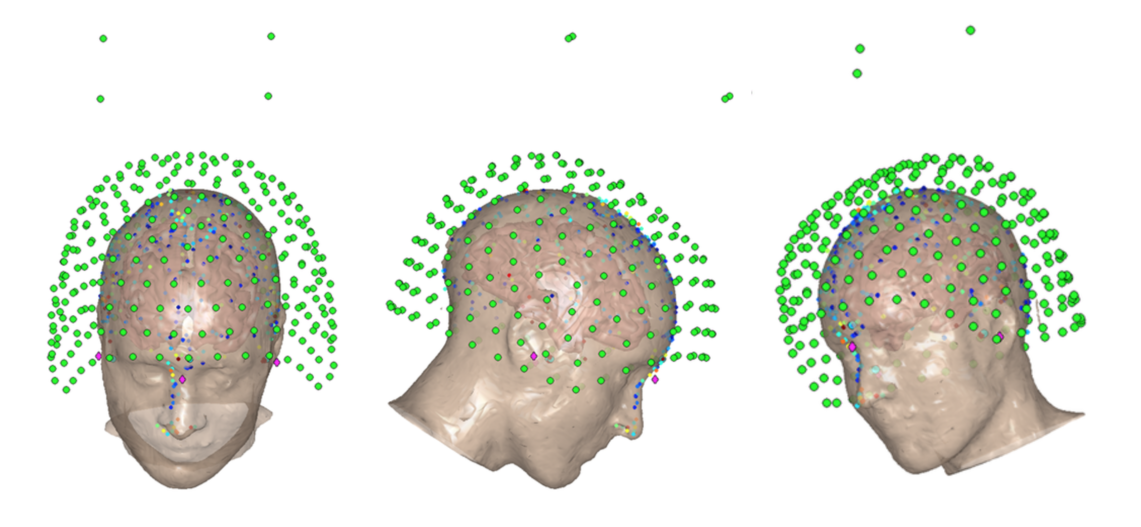
This SPM tool allows us to view the results of the coregistration (click and drag to rotate the image - you may need to click on the "Rotate 3D" toolbar button)

The coregistration shows several types of information:

figure('Position',[100 100 1024 1024])
spm_eeg_inv_checkdatareg_3Donly(spm_files_continuous);
zoom(0.5)

Coregistration with RHINO

To ensure a good coregistration we must make sure that the alignment between the MRI and Polhemus coordinates is as accurate as possible. There are several things we can do to improve on the typical pipeline:

RHINO is an OSL tool implementing these additional improvements. You need to make sure that you have a clear nose on your MRI scan and a large number of headshape points covering the scalp and ridgid parts of the face.

datadir = fullfile(osldir,'example_data','coreg_example');
spm_file=[datadir '/pdsubject1'];

S = [];
S.D = spm_file;
S.mri = fullfile(osldir,'example_data','coreg_example','subject1_struct_canon.nii');
S.useheadshape = 1;
S.use_rhino = 1; % We now set the RHINO option to 1
S.forward_meg = 'Single Shell';
S.fid.label.nasion = 'Nasion';
S.fid.label.lpa = 'LPA';
S.fid.label.rpa = 'RPA';
D=osl_headmodel(S);

Visualising structural preprocessing

The first time RHINO coregistration is run the structural data will be preprocessed using FSL tools. These perform a linear registration, brain extraction and scalp extraction from the T1 scan.

More information about RHINO can be found here:

https://ohba-analysis.github.io/osl-docs/pages/docs/preprocessing.html#coregistration-using-rhino

We can visualise the extracted scalp surface and original MRI scan in fsleyes with the following call.

This will load the structural scan overlayed on the scalp extraction. You can turn-off the strutural scan by double clicking on the picture of the eye to the left of the label 'subject1_struct_canon.nii' in the middle-bottom of the screen. Underneath, the scalp is the boundary between the white (outside) and black (inside) regions.

Try turning the structural scan on and off whilst exploring the image. There is a good correspondance between the scalp on the MRI and the extracted scalp image. Any deformations in the extracted scalp could be misleading when we align to our headshape points. In this case, the structrual preprcessing has worked well.

mri = fullfile(osldir,'example_data','coreg_example','rhino_subject1_struct_canon.nii');
scalp = fullfile(osldir,'example_data','coreg_example','rhino_subject1_struct_canon_scalp.nii.gz');

fsleyes({mri, scalp},[],'greyscale','none')

Visualising the RHINO coregistration

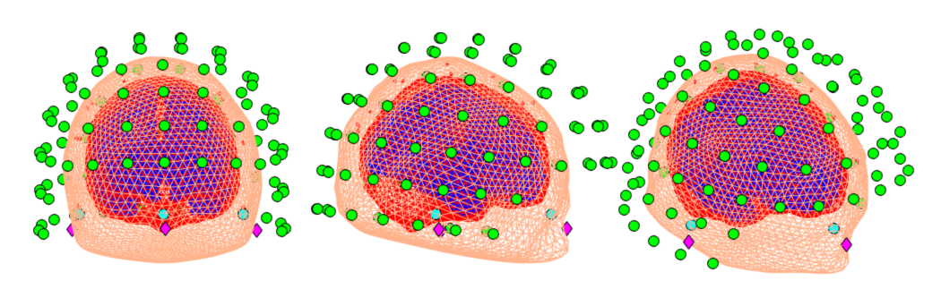
We can visualise the full coregistration by calling rhino_display(D).

This contains similar information to the SPM coreg.

You can click and drag the image to explore the registration.

Note the close correspondance between the headshape points and scalp extraction. The inclusion of the whole head and nose gives us greater confidence in the quality of the coregistration. Compare the RHINO surfaces with those from the SPM output.

This coregistration has worked very well. If you notice any large disparities in future analyses, these should be manually corrected at this stage:

D = spm_eeg_load(S.D);
rhino_display(D);

Published with MATLAB® R2018a