Utilities - Working with parcellations

This example shows how to use the OSL Parcellation object to work with parcellations.

Contents

Working with parcellations can be tedious, because there are several different ways to represent parcellations. Suppose we have a parcellation in MNI space on an 8mm grid. This space is codified in a standard mask - an anatomical brain image that defines the size of the space, and which grid coordinates are occupied by the brain. Although the space is defined on a regular grid, the brain only occupies a small subset of the volume. For example, in OSL the standard 8mm brain exists in a grid of size 23*27*23, but the brain only occupies 3559 voxels. A parcellation could be defined either in the volume (23*27*23) or in a vector of length equal to the number of voxels. Thus a parcellation with N parcels could be represented as

This is a complete representation of all possible parcellations. Note that parcels may be

In the case of a parcellation that is neither weighted nor overlapping, it is also possible to represent the parcellation using either a 'XYZ x 1' or 'Voxels x 1' matrix, where the value specifies which parcel the voxel belongs to. In this case, the matrix only has integer entries, and it is not possible to represent weighted or overlapping parcels. Thus there are 4 ways to represent parcellations. Converting between them requires the specification of a standard mask, which provides the mapping between voxel indices and MNI coordinates.

Thus, working with a parcellation requires keeping track of both the parcellation itself, and the standard mask. It may also involve changing the parcellation from one representation to another depending on what inputs are required by other analysis code. The Parcellation object aims to facilitate these steps.

To load a parcellation, create a parcellation object providing input as a '.nii' file. The .nii file should contain a matrix in one of the 4 supported sizes.

p = parcellation(fullfile(osldir,'parcellations','fmri_d100_parcellation_with_PCC_reduced_2mm_ss5mm_ds8mm.nii.gz'));

Alternatively, you can pass in a matrix in one of these supported formats

m = nii.load(fullfile(osldir,'parcellations','fmri_d100_parcellation_with_PCC_reduced_2mm_ss5mm_ds8mm.nii.gz'));
size(m)
p = parcellation(m);

ans =

    23    27    23    38

When the parcellation is loaded, two things happen

If you know the appropriate template mask, you can specify it manually (although this has not been extensively tested - many parcellations, and all of those supplied with OSL, work using the included standard mask files).

The Parcellation object displays some information about the loaded parcellation

p

p = 

  parcellation with properties:

             weight_mask: [23×27×23×38 double]
                  labels: {38×1 cell}
           template_mask: [23×27×23 double]
    template_coordinates: [3559×3 double]
          template_fname: '/Users/romesh/oxford_postdoc/toolboxes/osl/std_masks/MNI152_T1_8mm_brain.nii.gz'
             is_weighted: 1
          is_overlapping: 1
              resolution: 8
               n_parcels: 38
                n_voxels: 3559

If you want to specify the labels associated with the parcellation, you can do so by providing either a cell array of names for each region, or the name of a text file containing the name of each parcel on a separate line e.g.

% p = parcellation('my_parcellation.nii.gz',{'ROI 1','ROI 2'})
% p = parcellation('my_parcellation.nii.gz','my_parcellation_names.txt')

Reshaping matrices

One the most basic operations is converting between the XYZ x parcels and Voxels x parcels representations. You can do this with the to_matrix() and to_vol() methods. For example

matrix_representation = p.to_matrix(p.weight_mask);
size(matrix_representation)
volume_representation = p.to_vol(matrix_representation);
size(volume_representation)

ans =

        3559          38


ans =

    23    27    23    38

These functions also support an additional usage pattern. Often it is useful to visualize parcel-based data on the brain - for example, if you know the activation or spectral power at the parcel level. The data then consists of a vector, parcels x 1 (or 1 x parcels). Both to_matrix() and to_vol() can be given such a vector, which will then be expanded onto the voxels in either the matrix or volume representation.

expanded_volume = p.to_matrix(1:38);
size(expanded_volume)

Warning - parcellation is being binarized

ans =

        3559           1

Note that this can only be performed if the parcellation is binary (unweighted, with no overlap). If the parcellation does not meet these requirements, it will automatically be converted, and a warning will be displayed to indicate that this has occurred.

Finally, it also possible to convert the parcellation to the 'Voxels x 1' representation where value indicates parcel assignment

v = p.value_vector;
size(v)
v(end-10:end)

Warning - parcellation is being binarized

ans =

        3559           1


ans =

     0
     0
    27
    27
    28
     0
    27
    20
    20
    19
    20

Note that voxels that are not assigned to a parcel are given a value of 0.

MNI coordinates

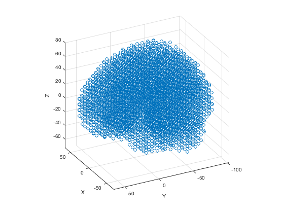
The MNI coordinates for the template are stored in the template_coordinates property.

size(p.template_coordinates)

ans =

        3559           3

See for example

figure
scatter3(p.template_coordinates(:,1),p.template_coordinates(:,2),p.template_coordinates(:,3))
axis equal
set(gca,'View', [-117.5000   26.8000])
xlabel('X');
ylabel('Y');
zlabel('Z');

The coordinates for each parcel can be obtained using the roi_coordinates method

r = p.roi_coordinates;

which returns a cell array of matrices, where each matrix contains the MNI coordinates for the voxels belonging to the parcel.

class(r)
size(r)
size(r{1})

ans =

    'cell'


ans =

     1    38


ans =

   129     3

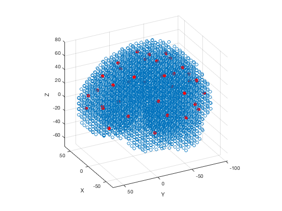
Finally, you can return the centre-of-mass of each parcel (the average of the ROI coordinates for voxels belonging to the parcel) using the roi_centres method

c = p.roi_centers;
c(1:3,:)
hold on
scatter3(c(:,1),c(:,2),c(:,3),50,'ro','filled')

ans =

  -10.0412  -87.3873   23.2642
   10.2322  -86.6912   23.1740
  -37.4042  -76.7157   -5.0137

Binarizing

We saw above that some operations required the parcellation to be binary. You can obtain the weight matrix corresponding to a binary parcellation using the binarize() function

binary_mask = p.binarize();

Binarization corresponds to first removing the overlap between parcels, by assigning them to a single parcel. This assignment is based on the voxel weights. For example, if voxel 1 belongs to parcel 1 (0.5) and parcel 2 (0.25), then it will be assigned to parcel 1. If you only wish to remove the overlap, use

no_overlap = p.remove_overlap();

This returns a weight matrix where the original weights are preserved, but there is no overlap. For example, here the new weights will be parcel 1 (0.5) and parcel 2 (0). To remove the weights, use

unweighted = p.remove_weights();

This returns a weight matrix where the overlap has not been removed, but the weights are binary. For example, for voxel 1 the new weights will be parcel 1 (1) and parcel 2 (1). Binarizing with binarize() corresponds to removing overlap, followed by removing weights (in that order).

If you want a new parcellation object based on the binarized weight matrix, you can simply construct a new parcellation object with the binary matrix as the input

binary_parcellation = parcellation(p.binarize)

binary_parcellation = 

  parcellation with properties:

             weight_mask: [23×27×23×38 double]
                  labels: {38×1 cell}
           template_mask: [23×27×23 double]
    template_coordinates: [3559×3 double]
          template_fname: '/Users/romesh/oxford_postdoc/toolboxes/osl/std_masks/MNI152_T1_8mm_brain.nii.gz'
             is_weighted: 0
          is_overlapping: 0
              resolution: 8
               n_parcels: 38
                n_voxels: 3559

Note how the binary parcellation has is_weighted=0 and is_overlapping=0.

Usage with ROI-nets

MEG-ROI-nets can compute parcel timecourses based on voxel timecourses, using methods such as PCA to reduce dimensionality. This functionality is provided through ROInets.get_node_tcs(). The parcellation needs to be passed in as a binary Voxels x parcels representation. As a shortcut, this can be obtained using the parcelflag() method. For example, to compute parcel timecourses from an SPM object, use

D = spm_eeg_load(fullfile(osldir,'example_data','roinets_example','subject_1.mat'));
D = D.montage('switch',2)
% D = ROInets.get_node_tcs(D,p.parcelflag,'PCA')

SPM M/EEG data object
Type: continuous
Transform: time
1 conditions
3559 channels
11251 samples/trial
1 trials
Sampling frequency: 250 Hz
Loaded from file  /Users/romesh/oxford_postdoc/toolboxes/osl/example_data/roinets_example/subject_1.mat

2 online montage(s) setup
Current montage applied (0=none): 2 ,named: "with weights normalisation, class 1"

Use the syntax D(channels, samples, trials) to access the data
Type "methods('meeg')" for the list of methods performing other operations with the object
Type "help meeg/method_name" to get help about methods

You might need to binarize and remove overlap in your parcellation to compute the parcel timecourses. You can do this by using p.parcelflag(true) where the first argument to parcelflag() specifies whether you would like to run binarize() internally or not. So if you had an overlapping, weighted parcellation, you might instead use

D2 = ROInets.get_node_tcs(D,p.parcelflag(true),'PCA')

get_node_tcs:    Finding PCA time course for ROI 1 out of 38

No new channels information : setting channels info automatically.
SPM M/EEG data object
Type: continuous
Transform: time
1 conditions
38 channels
11251 samples/trial
1 trials
Sampling frequency: 250 Hz
Loaded from file  /Users/romesh/oxford_postdoc/toolboxes/osl/example_data/roinets_example/subject_1.mat

3 online montage(s) setup
Current montage applied (0=none): 3 ,named: "Parcellated - with weights normalisation, class 1"

Use the syntax D(channels, samples, trials) to access the data
Type "methods('meeg')" for the list of methods performing other operations with the object
Type "help meeg/method_name" to get help about methods

Notice that the parcel timecourses are saved in the MEEG object as an online montage. This has been performed in memory, so you would need to run D2.save() to write the changes to disk.

Plotting and visualization in Matlab

The Parcellation object provides a number of options for plotting. To start with, the parcellation can be plotting using

p.plot

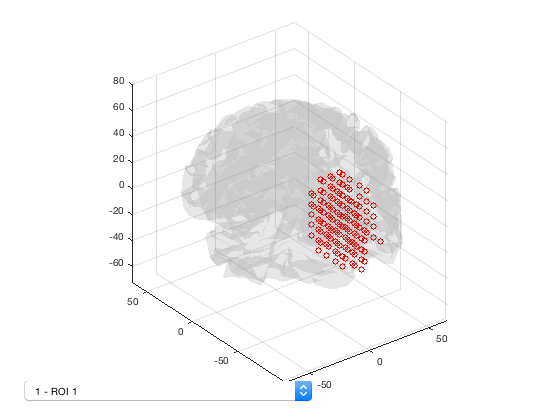
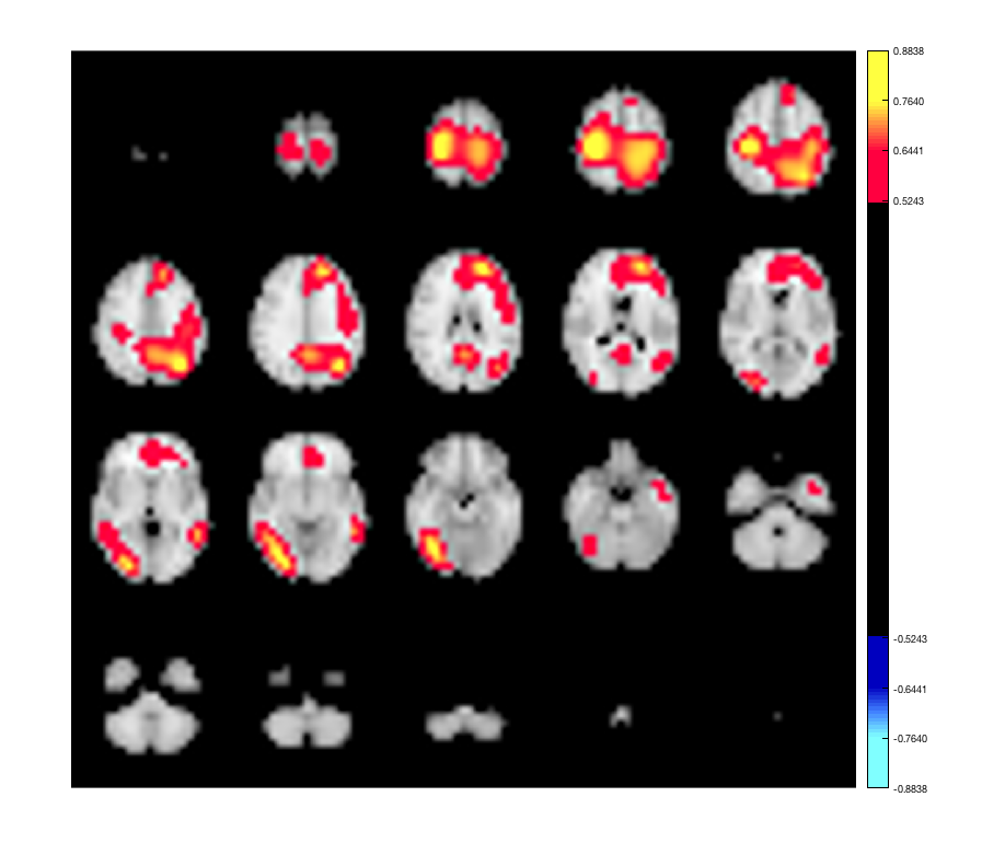
This displays a 3D plot of the parcellation. Each ROI can be selected from the dropdown list. It is also possible to show spatial maps of volume-wise activation - for example, a power map, or the activation map for an HMM state.

p.plot_activation(rand(size(p.template_mask)));

Warning: Image is too big to fit on screen; displaying at 67% 

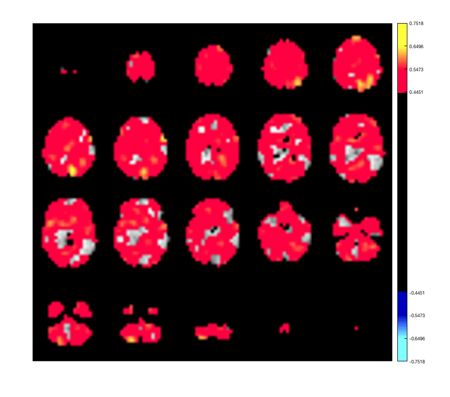
The input should be in XYZ x 1 format, but it will be automatically expanded if provided in Parcels x 1 format. For example

p.plot_activation(rand(p.n_parcels,1));

Warning - parcellation is being binarized
Warning: Image is too big to fit on screen; displaying at 67% 

Lastly, if you have a brain network connectivity matrix, you can display the strongest connections using the plot_network method. For example, to plot the top 5% of connections, you can use

connection_matrix = randn(p.n_parcels);
size(connection_matrix)
[h_patch,h_scatter] = p.plot_network(connection_matrix,0.95);

ans =

    38    38

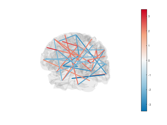
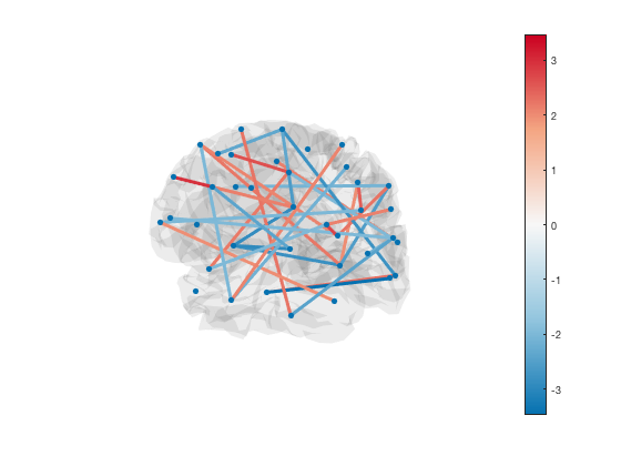
By default, the scatter plot is hidden with marker size NaN. To show the ROI centers, you can set the scatter plot marker size

set(h_scatter,'SizeData',30)

The line colours are matched to the colourmap. To change the colour scheme, simply adjust the colour range of the plot

set(gca,'CLim',[-1 1])

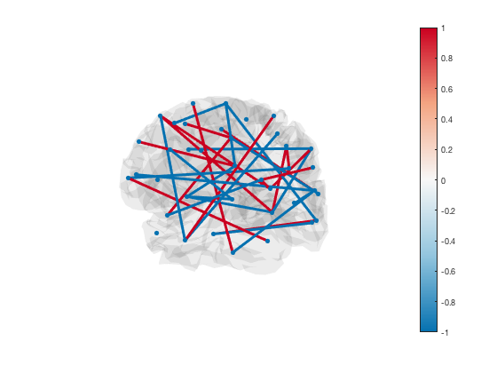
Finally, transparency is used to show or hide connections. Each edge has transparency equal to its percentile. You can adjust the alpha limits to change which connections are visible

set(gca,'ALim',[0 1]) % Show all connections
set(gca,'ALim',[0.9 1]) % Start fading in connections above 90th percentile
set(gca,'ALim',[0.95 0.95+1e-5]) % Hard cutoff at 95th percentile

Plotting using osleyes

There are a number of plotting options using osleyes. These can be accessed through the osleyes method. By default, this will display the parcellation with one volume for each parcel e.g.

p.osleyes

ans = 

  osleyes with properties:

             layer: [1×2 struct]
     current_point: [1 1 1]
      active_layer: 2
     show_controls: 1
    show_crosshair: 1
             title: ''
             nvols: 38
               fig: [1×1 Figure]
            images: {1×2 cell}

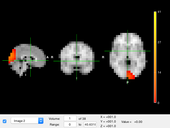
The osleyes method allows you to pass in a matrix to be displayed. For example,

p.osleyes(m)

ans = 

  osleyes with properties:

             layer: [1×2 struct]
     current_point: [1 1 1]
      active_layer: 2
     show_controls: 1
    show_crosshair: 1
             title: ''
             nvols: 38
               fig: [1×1 Figure]
            images: {1×2 cell}

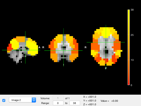
where the m matrix will be expanded into volume format if required. To plot all parcels in the same volume, you can use

p.osleyes(p.value_vector)

Warning - parcellation is being binarized

ans = 

  osleyes with properties:

             layer: [1×2 struct]
     current_point: [1 1 1]
      active_layer: 2
     show_controls: 1
    show_crosshair: 1
             title: ''
             nvols: 1
               fig: [1×1 Figure]
            images: {1×2 cell}

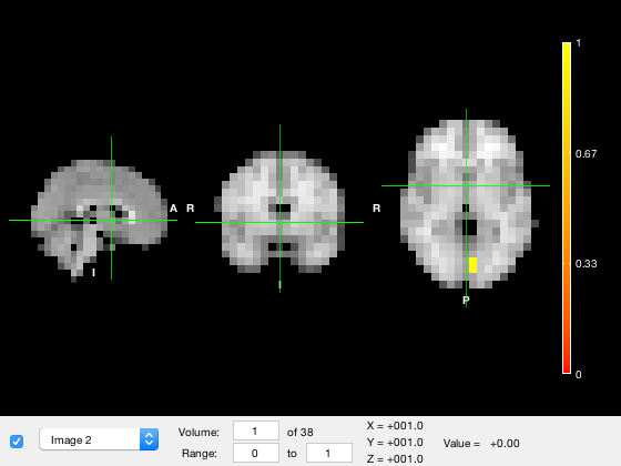
To plot the parcellation after binarization, you can use

p.osleyes(p.binarize)

ans = 

  osleyes with properties:

             layer: [1×2 struct]
     current_point: [1 1 1]
      active_layer: 2
     show_controls: 1
    show_crosshair: 1
             title: ''
             nvols: 38
               fig: [1×1 Figure]
            images: {1×2 cell}

Saving nii files

Lastly, and perhaps most importantly, you can save a matrix to a .nii file using

p.savenii(p.weight_mask,'filename')

ans =

    'filename.nii.gz'

this will create a file 'filename.nii.gz'. The weight mask is written directly into the .nii file, so it may only make sense if you pass in a volume. For example, to make a .nii file with the XYZ x 1 representation of the parcellation (value indices parcel membership) you could use

p.savenii(p.to_vol(1:38),'filename');

Warning - parcellation is being binarized

which will first expand the parcel assignments to each voxel.

Importantly, the savenii() method also copies the qform/xform portion of the header from the template mask into the newly saved file. This is important, partly because it specifies whether not the .nii file is saved in radiological orientation or not. Note that if the .nii file is missing this information, it may not be usable for some purposes.

Making surface plots

You can also use the parcellation class to render surface plots. This is performed via a call to Workbench. In order to use this functionality, you need to

If you have done both steps and run osl_startup, you should be able to type !wb_command in the command window, and see the usage information for the program. If not, you will need to fix your configuration before proceeding to make surface plots.

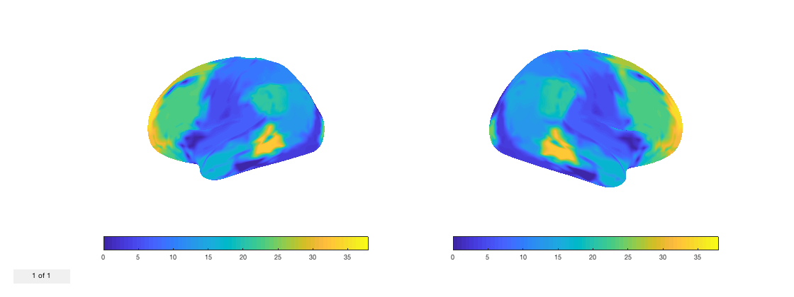
Making a surface plot is done using the plot_surface method of the parcellation object. Allowed inputs are the same as for osleyes, fsleyes, savenii etc. which means you can pass in voxel or parcel data in any supported matrix size. The data is automatically projected onto the cortical surface and rendered.

fig = p.plot_surface(1:38);

Warning - parcellation is being binarized

Note that the plot_surface method returns a handle to the figure. By default, the cortical surface is not inflated. You can select the inflation level by setting the second argument of plot_surface. The default value, 0, corresponds to no inflation. Otherwise, 1 corresponds to inflated, and 2 corresponds to very inflated.

p.plot_surface(1:38,2);

Warning - parcellation is being binarized

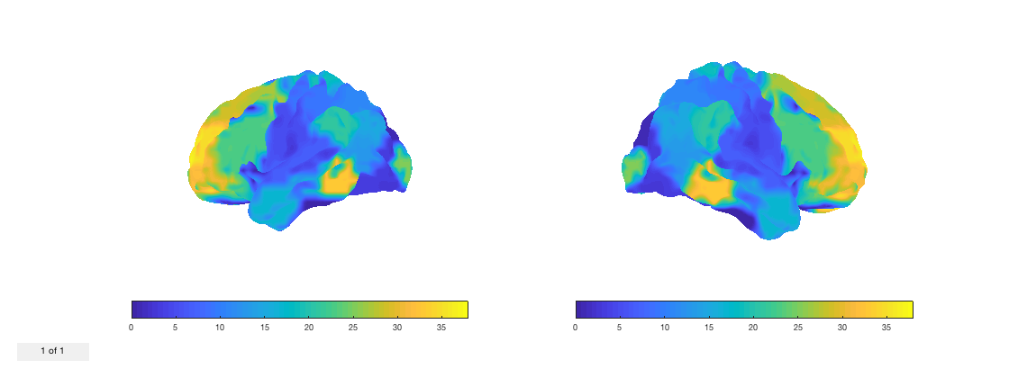
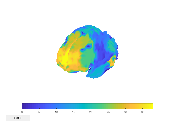
By default, the two hemispheres are shown separately. You can combine them into a single brain by setting the third option to true

p.plot_surface(1:38,[],true);
set(gca,'View',[-135 20]);

Warning - parcellation is being binarized

It's also possible to display multiple volumes. If your image contains an extra dimension (if you pass in a 2D or 4D matrix, such that to_vol would return a 4D matrix) then the plot will be generated with all volumes on the surface.

fig = p.plot_surface(randn(38,5));

Warning - parcellation is being binarized

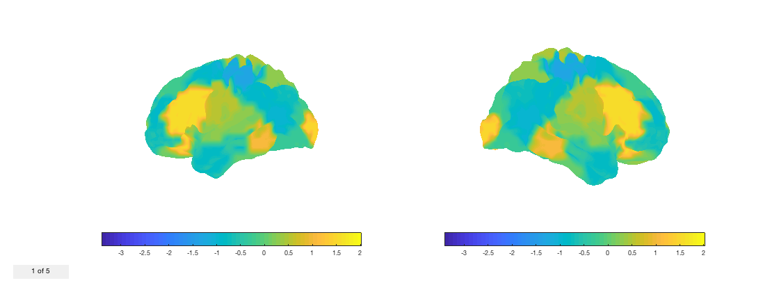
Notice that the count on the bottom left shows how many volumes are present. You can change the volume by using the buttons at the top of the window, or by setting the 'current_vol' property of the figure

fig.current_vol = 2;

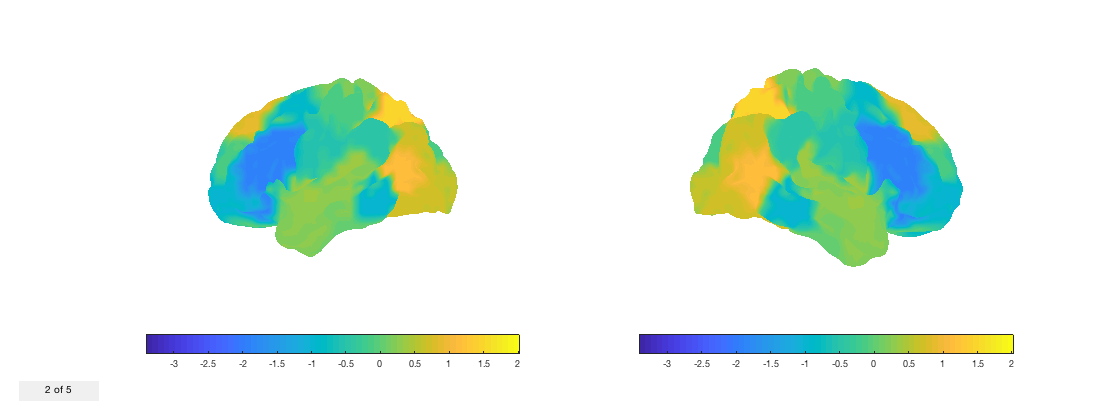
Let's put it together by rendering a time-varying tstat on the cortical surface. First, we need will take our voxelwise tstat and compute it at the parcel level.

nii_tstat = fullfile(osldir,'example_data','osleyes_example','tstat1_gc1_8mm.nii.gz');
d = nii.load(nii_tstat); % Load the data
d = p.to_matrix(d); % Convert to matrix form required by |ROInets|
d = ROInets.get_node_tcs(d,p.parcelflag,'SpatialBasis'); % Convert to parcel timecourses
fig = p.plot_surface(d,[],true); % Render on the surface
set(gca,'View',[-30 30]);
v = VideoWriter('parcellated_tstat.mp4','MPEG-4');
open(v)
for j = 1:size(d,2) % Iterate over volumes
    fig.current_vol = j;
    writeVideo(v,frame2im(getframe(fig)))
end
close(v)

Notice that the surface data is automatically interpolated by Workbench, so it is somewhat smoothed. You can set the interpolation type to any that is supported by wb_command by passing an additional argument to plot_surface.

Of course, we could do the same thing with the original voxel data without parcellating it. However, we would need to use a parcellation object for the original standard mask (i.e. with only one ROI encompassing all voxels). You could do this by just setting the parcel's weight mask to be the volume-version of the template mask, but for OSL standard masks, it's easiest just to specify the resolution you want.

p2 = parcellation(8);
d = nii.load(nii_tstat); % Load the data
fig = p2.plot_surface(d,[],true); % Render on the surface
set(gca,'View',[-30 30]);
v = VideoWriter('voxel_tstat.mp4','MPEG-4');
open(v)
for j = 1:size(d,4) % Iterate over volumes
    fig.current_vol = j;
    writeVideo(v,frame2im(getframe(fig)))
end
close(v)

Modifying parcellations

You can modify the parcellation simply by changing the weight matrix. For example

p.weight_mask(:,:,:,end+1) = p.weight_mask(:,:,:,end);

will duplicate the last parcel. Notice how the number of parcels has been updated

p.n_parcels

ans =

    39

Whether the parcellation is weighted or overlapping is automatically recomputed when you change the weight matrix.

Don't forget to add a new label as well! Some methods (such as removing or merging parcels below) require that the number of labels matches the number of parcels. This is enforced when you create the parcellation object, but is not checked if you manually edit the parcellation

p.labels{end+1} = 'New parcel';

You can easily remove parcels from the parcellation based on their index. For example, to remove the first 5 parcels, use

p2 = p.remove_parcels(1:5);
p2.n_parcels

ans =

    34

Note that this method returns a new parcellation with the specified parcels removed. This behaviour is the same as SPM MEEG objects.

You can also merge parcels. Merging is performed by adding the weight masks together for the specified parcels. If your parcellation is non-overlapping, the behaviour is obvious. If the parcellation does overlap, you should be aware that the weights are being combined additively. If this is not what you would like to do, you should just set the weight mask manually.

To merge parcels, specify a cell array with lists of parcels to merge. A new parcellation will be produced for each list in the cell array. All of the parcels that appear in the merge list will be removed from the parcellation. For example

p2 = p.merge_parcels({[1 2],[3 4]});

will create two new parcels, that are the composite of parcels 1 and 2, and parcels 3 and 4, AND the original parcels 1, 2, 3, and 4 will be removed. New labels are automatically created to reflect this.

p2.labels{1} % The first parcel is now ROI 5
p2.labels{end} % The last parcel is a composite of ROIs 3 and 4

ans =

    'ROI 5'


ans =

    'ROI 3+ROI 4'

Another operation that may be useful is splitting parcels. Currently this can be performed using k-means clustering of the voxel coordinates. To split parcels, use the split_parcels() method. The first argument is a list of parcels to split, and the second argument is the number of parcels to split it into. For example

p = parcellation(p.binarize);
p = p.remove_parcels(39); % Remove the last parcel, which has no voxels from the binarization
p2 = p.split_parcels([1 2],[3 4]);

will split the first parcel into 3 parts, and the second parcel into 4 parts. You can specify a scalar number of splits, which will be applied to every parcel, or you can leave the parcel list empty which will operate on all parcels e.g.

p3 = p.split_parcels([],2);

will split every parcel into two parts. The parcel names will be updated to reflect the splits.

Published with MATLAB® R2017a