Introduction to MEG Work Experience programme

This example script is designed to be used as part of a guided 1-hour overview of MEG analysis aimed at audiences with no/limited experience in neuroimaging (e.g. public). It is intended to be followed together with a presenter from OHBA who will cover complementary background content. The basic outline of the session is

Contents

Review of experimental task design

Your tutor will briefly review experimental task design, covering

Trial response, individual trials and averaging

First, we are going to load in the data files

abspath = @(s) fullfile(osldir,'example_data','intro_to_meg',s); % Get files relative to this path
oat = osl_load_oat(abspath('sensorspace_erf.oat'));
D = spm_eeg_load(abspath('meg_recording'));
response = @(sensor,trial) plot(D.time,mean(D(sensor,:,trial),3));
average_response = @(sensor) plot(D.time,mean(D(sensor,:,:),3));

Loaded OAT: /Users/romesh/oxford_postdoc/toolboxes/osl/example_data/intro_to_meg/sensorspace_erf.oat/oat_first_level_sub_level_group_level.mat
Data type is missing or incorrect, assigning default.

The variable D holds the MEG data. Have a look at what's in it

D

SPM M/EEG data object
Type: single
Transform: time
4 conditions
323 channels
751 samples/trial
360 trials
Sampling frequency: 250 Hz
Loaded from file  /Users/romesh/oxford_postdoc/toolboxes/osl/example_data/intro_to_meg/meg_recording.mat

Use the syntax D(channels, samples, trials) to access the data
Type "methods('meeg')" for the list of methods performing other operations with the object
Type "help meeg/method_name" to get help about methods

We can look at the response

response(10,5)

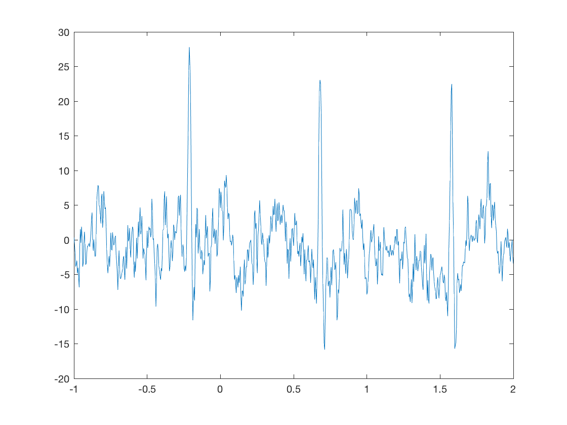
This means plot the signal from the 10th sensor, and the 5th trial. Note that there are three types of sensors

D.sensors('MEG').chantype(1:10)

ans =

  10×1 cell array

    'megplanar'
    'megplanar'
    'megmag'
    'megplanar'
    'megplanar'
    'megmag'
    'megplanar'
    'megplanar'
    'megmag'
    'megplanar'

Where are they?

pos = D.sensors('MEG').chanpos;
figure('Color','k','InvertHardCopy','off')
scatter3(pos(:,1),pos(:,2),pos(:,3),120,'b','filled')
hold on
for j = 1:3:size(pos,1)
	text(pos(j,1),pos(j,2),pos(j,3),num2str(j),'HorizontalAlignment','center','VerticalAlignment','middle','FontSize',12,'Color','w','FontWeight','bold');
end
axis equal
axis vis3d
axis off

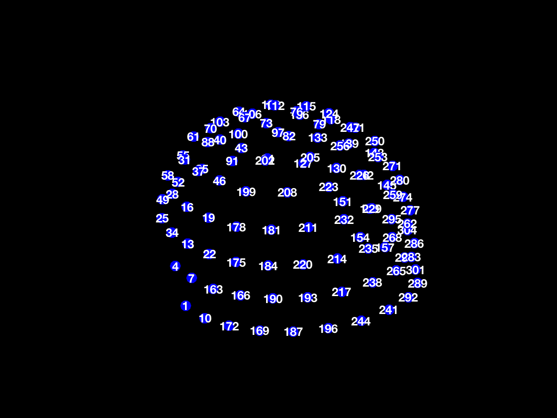
So each numbers on the plot corresponds to the first of three sensors at that location

ACTIVITIES

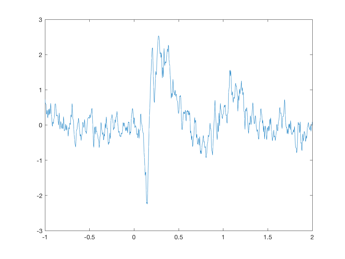
We can also look at the response, averaged over trials

figure
average_response(10)

ACTIVITIES

ACTIVITIES

Stats - COPEs and t-stats

Your tutor will present a brief overview of why statistical tests are used in the analysis, what COPEs and t-statistics are, and how to interpret them

Computing sensor stats

Now we are ready to look at some statistics. First, we need to find the location with the strongest response. Previously we did that by trial and error, but now we will do it systematically and automatically.

first_level_results=oat.first_level.results_fnames{1};
first_level_results=oat_load_results(oat,first_level_results);
first_level_cons_to_do=oat.first_level.report.first_level_cons_to_do; % plots all of these contrasts
S2=oat.first_level.report;
S2.stats=first_level_results;
S2.modality=oat.first_level.report.modality_to_do;
[vox_ind_max time_ind_max freq_ind_max stats max_stat] = oat_find_max_stats( S2 );

Next, plot the statistics over time. Note that the index of 'vox_ind_max' doesn't match the ones in the previous figure (see Activities to explore why this is the case)

S2=[];
S2.stats=stats;
S2.chanlabel=stats.chanlabels{vox_ind_max}; % can change to this setting to plot the time courses at the voxel with the max t-stat
S2.first_level_cons_to_do=first_level_cons_to_do;
[fig_handle fig_name fig_title] = oat_plot_vox_stats(S2);

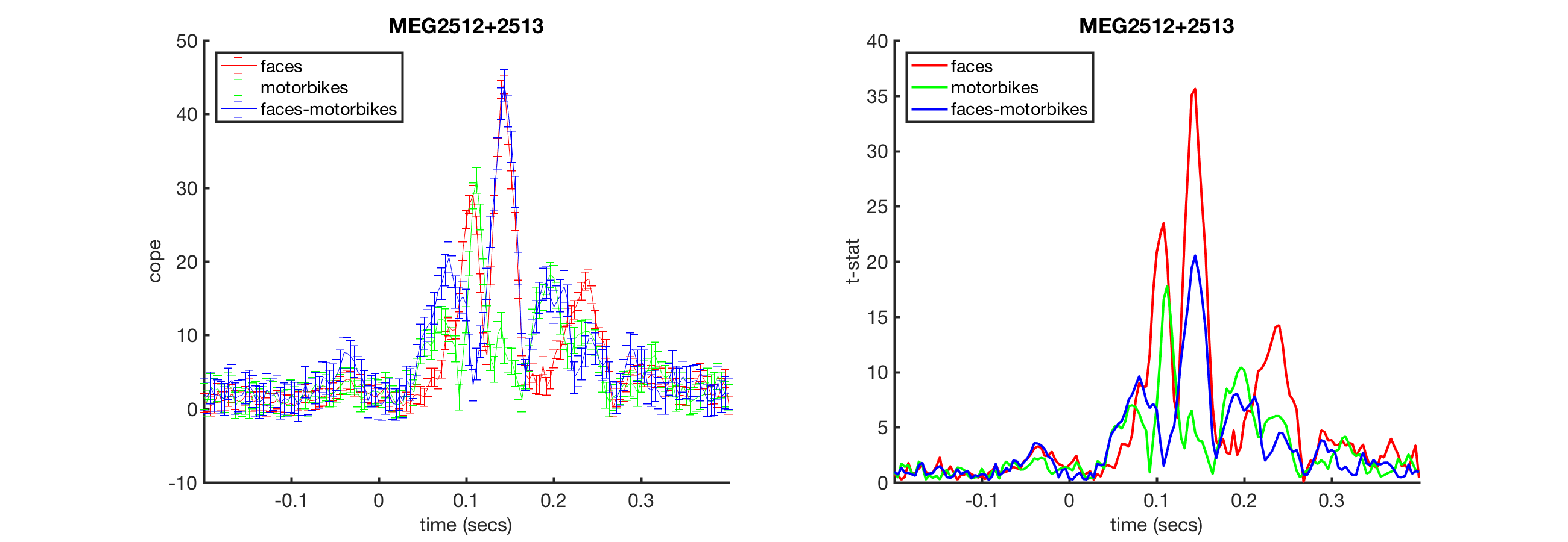
ACTIVITIES

Spatial variation in sensor task response

Next, we want a more systematic way to analyze the differences in space.

S2=[];
S2.oat=oat;
S2.stats_fname=oat.first_level.results_fnames{1};
S2.modality='MEGPLANAR'; % can also set this to 'MEGMAG'
S2.first_level_contrast=[3]; % view faces-motorbikes contrast
S2.view_cope=1; % set to 0 to see the t-stat
[cfg, dats, fig_handle]=oat_stats_multiplotER(S2);

Changing the number of channels, so discarding online montages.
Changing the number of channels, so discarding online montages.
selection avg along dimension 1
reading layout from file /Users/romesh/oxford_postdoc/toolboxes/osl/layouts/neuromag306cmb.lay

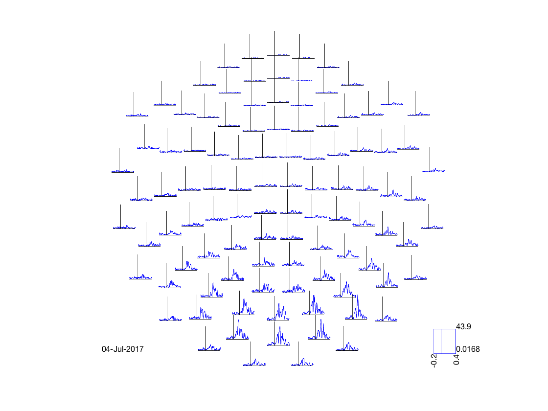
This plot is interactive * You can select sensors by drawing a box on the plot * You can then click inside the box to generate a time series obtained by averaging over all of the plots. * Finally, you can draw a box to select times on the plot, which will then be displayed on a 'topoplot' showing how they change over space

ACTIVITIES

Source space analysis: Concepts

Your tutor will briefly introduce the key concepts of source analysis

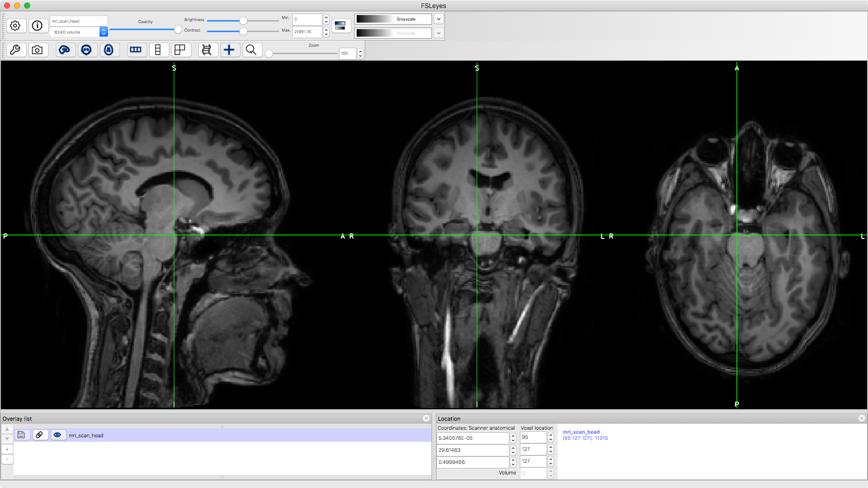
MRI structural scans

A critical step in beamforming is to quantify the position of the brain inside the head, in order to

First, we will take a look at a whole-head MRI scan.

runcmd('fsleyes %s',abspath('mri_scan_head.nii'))

ACTIVITIES * Trace visual pathway to V1 via thalamus * Find the cerebellum, and thalamus * Where is the grey matter? And the white matter? What does the white matter consist of?

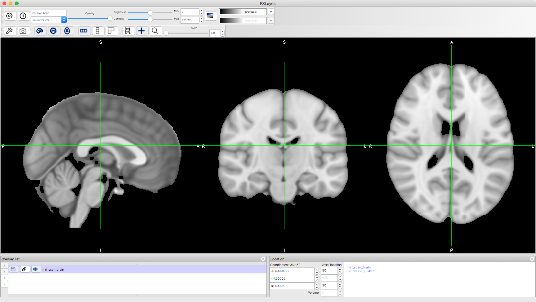
But usually, we're only interested in the brain. This second image is one that we are more used to, where the brain has been identified and extracted. This one is a 'standard brain' image, which is typically used for analysis after coregistration

runcmd('fsleyes %s',abspath('mri_scan_brain.nii.gz'))

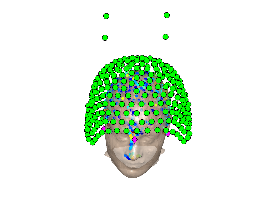
Coregistering MEG and MRI

The challenge in coregistration is to identify the brain inside the MEG scanner. Coregistration matches up the fiducial locations and the head shape data points with the MRI scan. We have software to automatically match them up. We can view the result of this process to check that the algorithm performed correctly

D = spm_eeg_load(abspath('rhino_example'));
D.inv{1}.mesh.sMRI = fullfile(osldir,'example_data','coreg_example','subject1_struct_canon.nii');
D.inv{1}.mesh.def = fullfile(osldir,'example_data','coreg_example','y_subject1_struct_canon.nii');
D.inv{1}.mesh.tess_ctx = fullfile(osldir,'example_data','coreg_example','subject1_struct_canoncortex_8196.surf.gii');
D.inv{1}.mesh.tess_scalp = fullfile(osldir,'example_data','coreg_example','subject1_struct_canonscalp_2562.surf.gii');
D.inv{1}.mesh.tess_oskull = fullfile(osldir,'example_data','coreg_example','subject1_struct_canonoskull_2562.surf.gii');
D.inv{1}.mesh.tess_iskull = fullfile(osldir,'example_data','coreg_example','subject1_struct_canoniskull_2562.surf.gii');
rhino_display(D);

Beamforming

Your tutor may wish to provide more information about beamforming at this point. However, it is sufficient to understand that the beamforming process takes place after coregistration.

Source space stats timecourses

Now we are in source space, we can ask what the timecourses look like for locations in the brain rather than for sensors.

oat = osl_load_oat(abspath('beamformer_erf.oat'),'wholebrain_first_level')
mni_coord=[32,-64,-18]; % Visual Cortex Voxel
S2=[];
S2.vox_coord=mni_coord;
S2.stats=oat.first_level.results_fnames{1};
S2.oat=oat;
S2.first_level_cons_to_do=oat.first_level.report.first_level_cons_to_do; % plots all of these contrasts
[vox_ind_used] = oat_plot_vox_stats(S2);

Loaded OAT: /Users/romesh/oxford_postdoc/toolboxes/osl/example_data/intro_to_meg/beamformer_erf.oat/oat_wholebrain_first_level_sub_level_group_level.mat

oat = 

  struct with fields:

            to_do: [1 1 0 0]
         do_plots: 0
     source_recon: [1×1 struct]
      first_level: [1×1 struct]
    subject_level: [1×1 struct]
      group_level: [1×1 struct]
     osl2_version: '1a3b6e0'
          results: [1×1 struct]
            fname: '/Users/romesh/oxford_postdoc/toolboxes/osl/example_data/intro_to_meg/beamformer_erf.oat/oat_wholebrain_first_level_sub_level_group_level.mat'

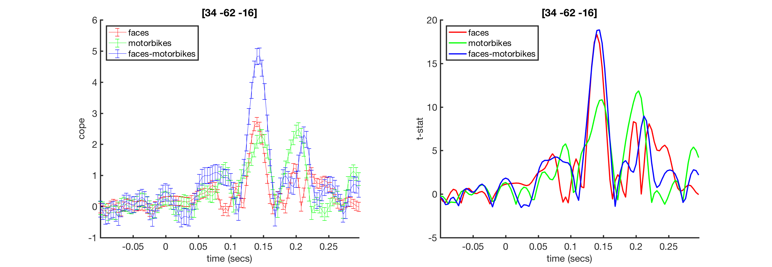
This will bring up a the COPE and tstat estimates across time for a voxel in visual cortex. Note the prominant response around 100ms

ACTIVITIES

Source-space spatial maps

As before, we might want an overview of where brain activity is in space. In sensor-space we did this using the topological plot. In source-space, we can do this using the brain scan itself.

fsleyes(abspath('beamformer_erf.oat/session1_wholebrain_first_level_dir/cope1_2mm.nii.gz'))

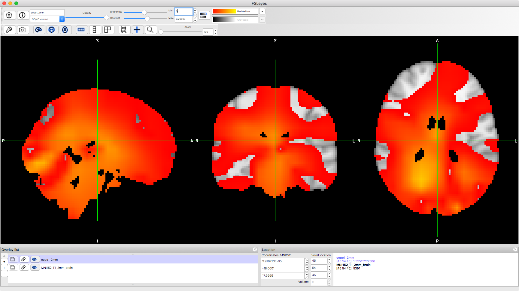
Note that you can change the colour range in the image to change which parts are displayed. In the first instance, it will be useful to change the lower limit to 0.

ACTIVITIES

Published with MATLAB® R2017a