OAT 4 - Group Analysis

This practical will work with a group-level OAT analysis run across 40 participants in the faces-motorbikes task we looked at in the single subject practical sessions.

Work your way through the script cell by cell using the supplied dataset. As well as following the instructions below, make sure that you read all of the comments (indicated by %), as these explain what each step is doing. Note that you can run a cell (marked by %%) using the Cell drop down menu on the Matlab GUI.

Contents

LOAD PRE-RUN GROUP OAT

A group analysis needs the source_recon, first_level and subject_level analyses to be completed for each participant and the group_level to be run across all the lower level results.

This takes quite a while to run for a 40 subject dataset, so to save time for this tutorial we have provided a completed OAT analysis which we can load in and explore.

This section loads the OAT analysis for which the first 3 stages (source recon, first-level GLM, subject-level averaging) have already been run. Note that the 1st level contrasts that have been run are:

% the directory containing the group OAT
workingdir = fullfile(osldir,'example_data','faces_group_data');

% Load in the previous OAT
oat = osl_load_oat(fullfile(osldir,'example_data','faces_group_data','beamform'), 'first_level_none','sub_level','group_level');

Loaded OAT: /Users/andrew/toolboxes/osl/example_data/faces_group_data/beamform.oat/oat_first_level_none_sub_level_group_level.mat

EXAMINE THE LOWER LEVEL ANALYSES

Take a look at the options for the source-recon and first-level analyses. These are very similar to the parameters we chose for the single subject ERF beamformer tutorial

Take a moment to familiarise yourself with the options. In particular, look at the first level GLM settings and which contrasts have been run. This can be found in oat.first_level.contrast and oat.first_level.contrast_name.

disp(oat.source_recon);
disp(oat.first_level);

                time_range: [-0.1500 0.3000]
                conditions: {1×4 cell}
              D_continuous: []
                 D_epoched: {1×14 cell}
                freq_range: [1 48]
                   dirname: '/Users/andrew/toolboxes/osl/example_data/faces_group_data/beamform.oat'
            sessions_to_do: 3
                 epochinfo: []
                    method: 'beamform'
     bandstop_filter_mains: 0
        artefact_chanlabel: []
                modalities: {'MEGPLANAR'  'MEGMAG'}
             session_names: {14×1 cell}
          normalise_method: 'mean_eig'
                     regpc: 0
                  gridstep: 9
               forward_meg: 'Single Shell'
                       mri: {1×28 cell}
                   pca_dim: [14×1 double]
             force_pca_dim: 1
                      type: 'Scalar'
            hmm_num_states: 0
            hmm_num_starts: 1
               hmm_pca_dim: 40
    hmm_av_class_occupancy: 35
                    report: [1×1 struct]
            results_fnames: {14×1 cell}

                                     doGLM: 1
                     design_matrix_summary: {1×4 cell}
                                  contrast: {1×3 cell}
                             contrast_name: {1×3 cell}
                            sessions_to_do: 3
                                time_range: [-0.1500 0.3000]
                         baseline_timespan: [-0.1500 0]
                  do_weights_normalisation: 1
                            use_robust_glm: 0
                                        bc: [3×1 double]
              sensor_space_combine_planars: 'combine_cartesian'
                              bc_trialwise: 0
                                      name: 'first_level_none'
                   time_moving_av_win_size: []
          post_glm_time_moving_av_win_size: []
                      hmm_do_glm_statewise: 0
                                 tf_method: 'none'
                             tf_freq_range: [1 48]
                              tf_num_freqs: 1
                              time_average: 0
                     tf_multitaper_ncycles: []
      post_movingaverage_downsample_factor: []
                 post_tf_downsample_factor: []
                       tf_hilbert_freq_res: 2
    tf_hilbert_do_bandpass_for_single_freq: 0
                    tf_hilbert_freq_ranges: []
                          tf_morlet_factor: 6
                        tf_hanning_ncycles: []
                                 cope_type: 'acope'
                       save_trialwise_data: 0
                       trialwise_directory: []
                              parcellation: [1×1 struct]
                                is_epoched: 1
                             do_glm_demean: 0
                                    report: [1×1 struct]
                               warp_fields: []
                            results_fnames: {14×1 cell}

SUBJECT LEVEL OPTIONS

The subject level allows for a fixed-effects combination of different datasets recorded from a single participant. To clarify some terminology:

If we have a design in which one subject has contributed several sessions, we can combine the COPEs from each session to get a subject level estimate. This subject level estimate is then passed into the group_level analysis.

The key parameter in the subject level is oat.subject_level.session_index_list. This is a cell array with a cell containing the indices of all the first_level sessions contributed by that subject.

There are some extra options for computing laterality contrasts at the subject level. This is useful if you was to compare a response or effect between the left and right hemispheres. For instance, is the response to a tactile stimulation on the hand larger in the ipsi or contra lateral hemisphere?

In our case, each subject contributed a single session so this indexing is a simple one-to-one matching between the first_level and subject_level

disp(oat.subject_level);
disp(oat.subject_level.session_index_list);

    session_index_list: {1×14 cell}
        subjects_to_do: [1 2 3 4 5 6 7 8 9 10 11 12 13 14]
                  name: 'sub_level'
    compute_laterality: []
      merge_contraipsi: []
        results_fnames: {14×1 cell}

  Columns 1 through 11

    [1]    [2]    [3]    [4]    [5]    [6]    [7]    [8]    [9]    [10]    [11]

  Columns 12 through 14

    [12]    [13]    [14]

SETUP GROUP-LEVEL OPTIONS

This section defines the parameters for the group_level in the OAT analysis.

The group design matrix is defined as a single vector of ones, this calculates a group average across all participants. Finally the first-level and group-level contrasts to run for the report are set up. In this case we are running first level contrast 3 (faces > motorbikes) and group level contrast 1 (grand mean).

oat.group_level.name='group_level';
oat.group_level.subjects_to_do=[1:14];

% Spatial and temporal averaging options
oat.group_level.time_range=[-0.1 0.3];
oat.group_level.space_average=0;
oat.group_level.time_average=0;
oat.group_level.time_smooth_std=0; % secs
oat.group_level.use_tstat=0;

% Spatial and temporal smoothing options
oat.group_level.spatial_smooth_fwhm=0; % mm
oat.group_level.group_varcope_time_smooth_std=100;
oat.group_level.group_varcope_spatial_smooth_fwhm=100; % smooths the variance of the group copes. It is recommended to do this.

% Set up design matrix and contrasts
oat.group_level.group_design_matrix=ones(1,length(oat.group_level.subjects_to_do));
oat.group_level.group_contrast=[];
oat.group_level.group_contrast{1}=[1]';
oat.group_level.group_contrast_name={};
oat.group_level.group_contrast_name{1}='mean';

% Define which contrasts to perform for the report
oat.group_level.first_level_contrasts_to_do=[1:3]; % list of first level contrasts to run the group analysis on
oat.group_level.report.first_level_cons_to_do=[2,1,3]; % purely used to determine which contrasts are shown in the report, the first one in list determines the contrast used to find the vox, time, freq with the max stat
oat.group_level.report.group_level_cons_to_do=[1]; % purely used to determine which contrasts are shown in the report, the first one in list determines the contrast used to find the vox, time, freq with the max stat
oat.group_level.report.show_lower_level_copes=0;
oat.group_level.report.show_lower_level_cope_maps=0;

CHECK OAT

The OAT structure that we have created should be passed to osl_run_oat to perform the pipeline as defined. However the OAT structure should also contain oat.to_do which is a list of binary values indicating which stages of the OAT to run.

The OAT analysis we loaded at the start of this practical has already been run for you (due to long computation time), so we do not need actually re-run the OAT here. In practice, we would call osl_run_oat after osl_check_oat to run the analysis.

oat.to_do=[0 0 0 1]; % run group-level stage only

oat = osl_check_oat( oat );

oat = osl_run_oat( oat );

Unknown datatype. Using default Elekta Neuromag 306 settings
Warning: oat.source_recon.modalities not set, or not set properly. Will set to
default:MEGPLANARMEGMAG 
oat.source_recon.D_epoched set. OAT will do an epoched data trial-wise GLM
Unknown datatype. Using default Elekta Neuromag 306 settings
Warning: oat.source_recon.modalities not set, or not set properly. Will set to
default:MEGPLANARMEGMAG 
oat.source_recon.D_epoched set. OAT will do an epoched data trial-wise GLM
*************************************************************
Running group_level
*************************************************************
Loading in lower level stats
Using same indices as lower_level
 - estimated time to finish is 0 seconds
Processing Group stats for first level contrast 1, motorbikes
Number 1 of 3
Preparing data
Computing group statistics
 - estimated time to finish is 0 seconds
Do spatial smoothing of group varcopes with FWHM=100 mm
Processing Group stats for first level contrast 2, faces
Number 2 of 3
Preparing data
Computing group statistics
 - estimated time to finish is 0 seconds
Do spatial smoothing of group varcopes with FWHM=100 mm
Processing Group stats for first level contrast 3, faces-motorbikes
Number 3 of 3
Preparing data
Computing group statistics
 - estimated time to finish is 0 seconds
Do spatial smoothing of group varcopes with FWHM=100 mm
Processing Group stats for first level contrast 2 [faces]
Number 1 of 3
Outputting nii files for first level contrast 2
E.g. to view nii file: 
fsleyes('/Users/andrew/toolboxes/osl/example_data/faces_group_data/beamform.oat/plots/first_level_none_sub_level_group_level/tstat2_gc1_2mm.nii.gz')
Processing Group stats for first level contrast 1 [motorbikes]
Number 2 of 3
Outputting nii files for first level contrast 1
E.g. to view nii file: 
fsleyes('/Users/andrew/toolboxes/osl/example_data/faces_group_data/beamform.oat/plots/first_level_none_sub_level_group_level/tstat1_gc1_2mm.nii.gz')
Processing Group stats for first level contrast 3 [faces-motorbikes]
Number 3 of 3
Outputting nii files for first level contrast 3
E.g. to view nii file: 
fsleyes('/Users/andrew/toolboxes/osl/example_data/faces_group_data/beamform.oat/plots/first_level_none_sub_level_group_level/tstat3_gc1_2mm.nii.gz')
To view group level report, point your browser to <a href="/Users/andrew/toolboxes/osl/example_data/faces_group_data/beamform.oat/plots/first_level_none_sub_level_group_level/report.html">/Users/andrew/toolboxes/osl/example_data/faces_group_data/beamform.oat/plots/first_level_none_sub_level_group_level/report.html</a>
Saving statistics in file /Users/andrew/toolboxes/osl/example_data/faces_group_data/beamform.oat/first_level_none_sub_level_group_level
To create niftii files from this use a call to oat_save_nii_stats
To view group level report, point your browser to <a href="/Users/andrew/toolboxes/osl/example_data/faces_group_data/beamform.oat/plots/first_level_none_sub_level_group_level/report.html">/Users/andrew/toolboxes/osl/example_data/faces_group_data/beamform.oat/plots/first_level_none_sub_level_group_level/report.html</a>
To view OAT report, point your browser to <a href="/Users/andrew/toolboxes/osl/example_data/faces_group_data/beamform.oat/plots/report.html">/Users/andrew/toolboxes/osl/example_data/faces_group_data/beamform.oat/plots/report.html</a>

CREATE A STATS REPORT

We will create a stats report (without rerunning OAT), where we look for the maximum stat for a different first level contrast (specified by S.first_level_con), within the time range S.time_range:

oat.results.plotsdir =fullfile(osldir,'example_data','faces_group_data','beamform.oat','plots');

oat.group_level.report.time_range=[0.07 0.13];
oat.group_level.report.first_level_cons_to_do=[2,1,3]; % purely used to determine which contrasts are shown in the report, the first one in list determines the contrast used to find the vox, time, freq with the max stat
oat.group_level.report.group_level_cons_to_do=[1]; % we want to isolate the group average response
oat.group_level.report.show_lower_level_cope_maps=0; %
report = oat_group_level_stats_report(oat,oat.group_level.results_fnames);

Processing Group stats for first level contrast 2 [faces]
Number 1 of 3
Outputting nii files for first level contrast 2
E.g. to view nii file: 
fsleyes('/Users/andrew/toolboxes/osl/example_data/faces_group_data/beamform.oat/plots/first_level_none_sub_level_group_level/tstat2_gc1_2mm.nii.gz')
Processing Group stats for first level contrast 1 [motorbikes]
Number 2 of 3
Outputting nii files for first level contrast 1
E.g. to view nii file: 
fsleyes('/Users/andrew/toolboxes/osl/example_data/faces_group_data/beamform.oat/plots/first_level_none_sub_level_group_level/tstat1_gc1_2mm.nii.gz')
Processing Group stats for first level contrast 3 [faces-motorbikes]
Number 3 of 3
Outputting nii files for first level contrast 3
E.g. to view nii file: 
fsleyes('/Users/andrew/toolboxes/osl/example_data/faces_group_data/beamform.oat/plots/first_level_none_sub_level_group_level/tstat3_gc1_2mm.nii.gz')
To view group level report, point your browser to <a href="/Users/andrew/toolboxes/osl/example_data/faces_group_data/beamform.oat/plots/first_level_none_sub_level_group_level/report.html">/Users/andrew/toolboxes/osl/example_data/faces_group_data/beamform.oat/plots/first_level_none_sub_level_group_level/report.html</a>

VIEW GROUP LEVEL STATS REPORT

Click the link to open the stats report after the previous cell has completed.

The report shows a range of plots which are useful for checking the analysis has run properly and summarising the key results.

On first page we see:

Group-level design matrix - This is the GLM design matrix from our analysis

Average lower level STDCOPEs - These show the variance of the COPE estimate averaged over time for each subject for each contrast. If any subject has an extremely high or low variance it might indicate that their are an outlier and we should double check their lower level results. Perhaps they have very few good trials in one condition or their coregistration has gone wrong.

Stats for GC1 - These are the group average COPEs and t-stats for the lower level contrasts.

Lower level COPES - These show the COPES for each individual subject for each lower-level contrast. The thick line indicates the group mean. Again it is good to check these to identify any outlier subject.

Lower-level STDCOPES - These are the lower-level COPEs (as we saw above) from the maximal time-point in the faces contrast.

There are no apparent outliers in our diagnostic plots so we can click the links at the top of the page to explore the group results for each of the lower level contrasts in more detail.

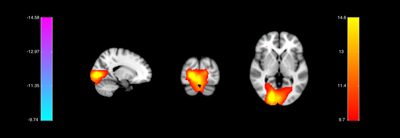
Click the link to open the results for the faces contrast.

Here we see the group level COPE and t-stats across the brain for the faces contrast. The time-point is chosen by the maximum response in the faces condition. There is a clear occipital response around 100ms after stimulus onset. Explore the results from the other contrasts before moving on to the next cell.

OUTPUT GROUP'S NIFTII FILES

As with the single subject analyses we can output nifti files containing the group-level results across the whole brain and the whole experimental epoch.

This section saves out a nifti volume containing the results from first_level contrast 3 (faces > motorbikes) across the whole group

S2=[];
S2.oat=oat;
S2.stats_fname=oat.group_level.results_fnames;
S2.first_level_contrasts=[3,2,1]; % list of first level contrasts to output
S2.group_level_contrasts=[1]; % we want to isolate the group average response
S2.resamp_gridstep=8;
[statsdir,times]=oat_save_nii_stats(S2);

Outputting nii files for first level contrast 3
Outputting nii files for first level contrast 2
Outputting nii files for first level contrast 1
E.g. to view nii file: 
fsleyes('/Users/andrew/toolboxes/osl/example_data/faces_group_data/beamform.oat/first_level_none_sub_level_group_level_dir/tstat1_gc1_8mm.nii.gz')

VIEW NIFTII RESULTS IN OSLEYES

Run the code below to open OSLEYES with the group-level results for the faces-motorbikes contrast along with a structural image and a mask of the right hemisphere fusiform cortex.

tstat = fullfile( oat.source_recon.dirname,'first_level_none_sub_level_group_level_dir','tstat3_gc1_8mm.nii.gz' );
fusiform = fullfile(osldir,'example_data','faces_group_data','structurals','Right_Temporal_Occipital_Fusiform_Cortex_8mm.nii.gz');
o = osleyes({[],tstat,fusiform},'clim',{[],[5 8],[0 5]},'colormap',{[],osl_colormap('hot'),osl_colormap('green')})

o = 

  osleyes with properties:

             layer: [1×3 struct]
     current_point: [1 1 1]
      active_layer: 3
     show_controls: 1
    show_crosshair: 1
             title: ''
             nvols: 1
               fig: [1×1 Figure]
            images: {1×3 cell}

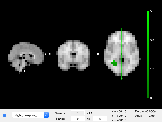
Explore the volume to find the green Fusiform Mask. This is brain region which is closely associated with the processing of visual information and is particularly specialised for processing faces.

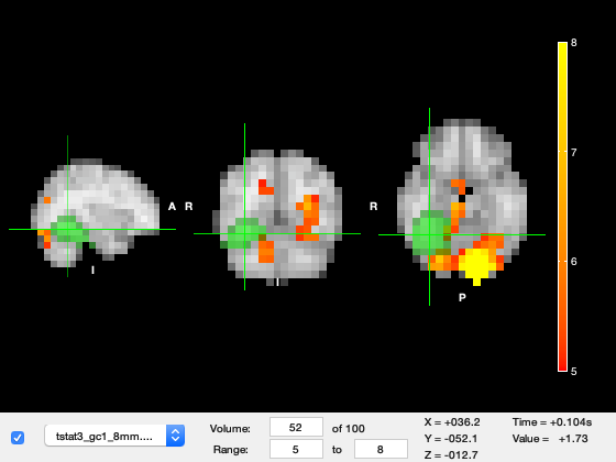
Make sure the tstat3_gc1_8mm layer is selected in the dropdown menu. We will make the ROI translucent so that it can be viewed at the same time as the activation.

o.active_layer = 2; % Select tstat layer
o.layer(3).alpha = 0.5; % Make ROI transparent
o.current_point = [36.1579 -52.1053 -12.7368]; % Position the image at the ROI

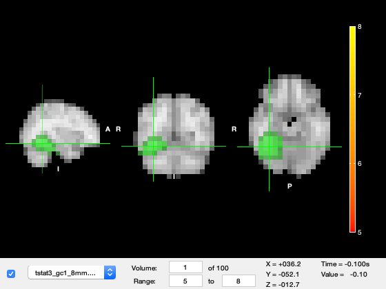
Change the Volume in the bottom left to 52, this corresponds to about 100ms after stimulus onset. We can see a very strong response in primary visual cortex in the medial part of the occipital lobes.

o.layer(2).volume = 52;

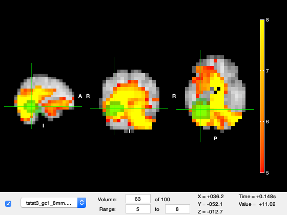
Now change the Volume to 63, this corresponds to ~150ms after stimulus onset. The primary visual response has finished and now the region highlighted by the Green fusiform mask has a much stronger response.

o.layer(2).volume = 63;

INVESTIGATING LOCATIONS OF INTEREST USING AN MNI COORDINATE

In this section we will interrogate the wholebrain OAT (run above) using an MNI coordinate of interest.

First, you need to specify the MNI co-ordinate of the location of interest and use this MNI coordinate to set the parameter, mni_coord

Now run that cell. This loads in the wholebrain OAT and its results, finds the results that correspond to the MNI coordinate of interest, and finally, plots the time-courses of the statistics for the different contrasts at the MNI coordinate specified.

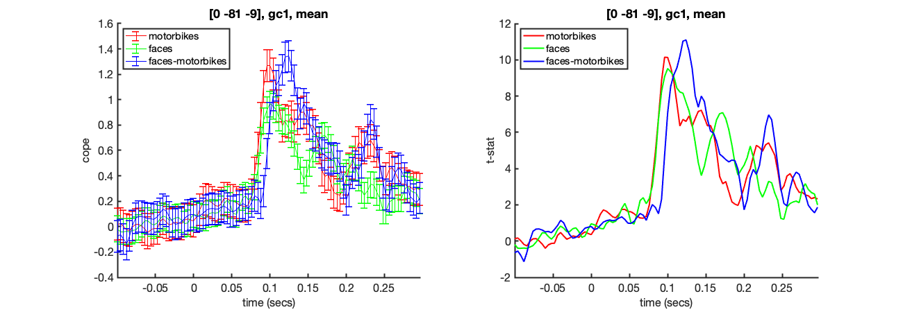
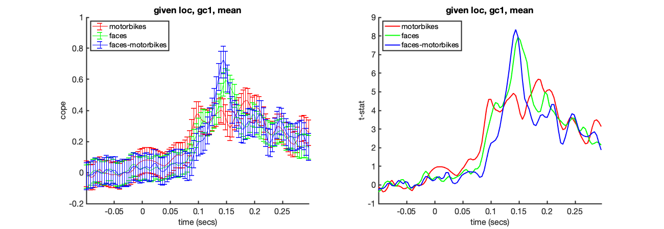
We can isolate the results from a specific voxel using oat_plot_vox_stats. Here we will look at the group results for all three lower level contrasts in the visual cortex.

Once you have run this once, try changing the co-ordinate to 32,-64,-18. What differences do you notice?

mni_coord=[4,-82,-8];

S2=[];
S2.oat=oat;
S2.stats=oat.group_level.results_fnames;
S2.vox_coord=mni_coord;
S2.first_level_cons_to_do = [2,1,3];
S2.group_level_cons_to_do = [1];
oat_plot_vox_stats(S2);

INVESTIGATING REGIONS OF INTEREST USING AN MNI MASK

In this section we will interrogate the wholebrain OAT (run above) using an ROI mask. This will provide the results averaged across all voxels in the defined mask.

In particular, note the setting S2.mask_fname which specifies the mask to be used. This spatially averages over the ROI, and plots the timecourses of the statistics for the different contrasts.

We will use the right hemisphere Fusiform Cortex mask which we used previouly.

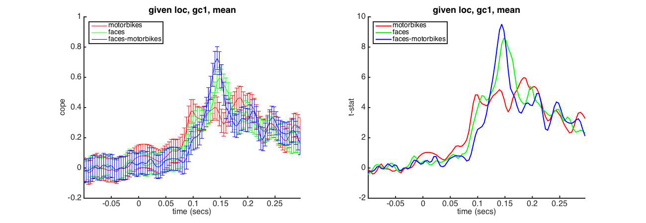
% load OAT analysis for which the first 4 stages have already been run
oat = osl_load_oat(fullfile(osldir,'example_data','faces_group_data','beamform'), 'first_level_none','sub_level','group_level');

% Spatially average the results over an ROI
S2=[];
S2.oat=oat;
S2.stats_fname=oat.group_level.results_fnames;
S2.mask_fname=fullfile(osldir,'example_data','faces_group_data','structurals','Right_Temporal_Occipital_Fusiform_Cortex_8mm.nii.gz');
[stats,times,mni_coords_used]=oat_output_roi_stats(S2);

% plot
S2=[];
S2.stats=stats;
S2.oat=oat;
S2.first_level_cons_to_do = [2,1,3];
S2.group_level_cons_to_do = [1];
[vox_ind_used] = oat_plot_vox_stats(S2);

Loaded OAT: /Users/andrew/toolboxes/osl/example_data/faces_group_data/beamform.oat/oat_first_level_none_sub_level_group_level.mat

GROUP STATS ON A SINGLE VOLUME WITHIN A TIME-WINDOW

Here we will run the group GLM on an average of the first-level data between the times 140 ms and 150 ms. This will produce a single volume for viewing in fslview.

Note that we have specified a time range of 140-150ms, and specified that we want to average over the time window with the setting:

Now run the cell, which should also open fslview for you to view the results.

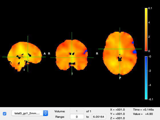
Unlike earlier, there will now just be a single volume (time point) averaged over the specified time range of 140-150ms. To view the results properly, setup appropriate color-maps for the images and threshold the t-stat at about 4.5, and the cope at about 0.005.

Once you have run this cell, try re-running to look at the window between 90 and 120 ms after stimulus onset. What differences do you notice between the early (90-120ms) and later (140-150ms) responses?

% load in OAT with first 3 stages run:

% specify the time-range to average over
oat.group_level.time_range=[0.140 0.150];
oat.group_level.time_average=1;

oat.group_level.first_level_contrasts_to_do=[1:3]; % list of first level contrasts to run the group analysis on
oat.group_level.report.first_level_cons_to_do=[3]; % purely used to determine which contrasts are shown in the report, the first one in list determines the contrast used to find the vox, time, freq with the max stat
oat.group_level.report.group_level_cons_to_do=[1]; % purely used to determine which contrasts are shown in the report, the first one in list determines the contrast used to find the vox, time, freq with the max stat

oat.group_level.name='time_average_group_level';
oat.group_level.use_tstat=0;
oat.group_level.group_varcope_spatial_smooth_fwhm=100;

% Check and run the OAT analysis
oat = osl_check_oat(oat);
oat.to_do=[0 0 0 1];
oat = osl_run_oat(oat);

% Output the single volume results
S2=[];
S2.oat=oat;
S2.stats_fname=oat.group_level.results_fnames;
S2.first_level_contrasts = [2,1,3];
S2.group_level_contrasts = [1];

[statsdir,times]=oat_save_nii_stats(S2);

% View the single volume results
con=3;
gcon=1;

tstat = fullfile(statsdir,['tstat' num2str(con) '_gc' num2str(gcon) '_2mm.nii.gz']);
cope  = fullfile(statsdir,['cope' num2str(con) '_gc' num2str(gcon) '_2mm.nii.gz' ]);

osleyes( {[],cope,tstat} );

Unknown datatype. Using default Elekta Neuromag 306 settings
Warning: oat.source_recon.modalities not set, or not set properly. Will set to
default:MEGPLANARMEGMAG 
oat.source_recon.D_epoched set. OAT will do an epoched data trial-wise GLM
Unknown datatype. Using default Elekta Neuromag 306 settings
Warning: oat.source_recon.modalities not set, or not set properly. Will set to
default:MEGPLANARMEGMAG 
oat.source_recon.D_epoched set. OAT will do an epoched data trial-wise GLM
*************************************************************
Running group_level
*************************************************************
Loading in lower level stats
Using same indices as lower_level
 - estimated time to finish is 0 seconds
Processing Group stats for first level contrast 1, motorbikes
Number 1 of 3
Preparing data
Warning: Doing time averaging. This means that there will be no variance
smoothing of the between-subject variance (as specified by
group_varcope_time_smooth_std). 
Computing group statistics
 - estimated time to finish is NaN seconds
Do spatial smoothing of group varcopes with FWHM=100 mm
Processing Group stats for first level contrast 2, faces
Number 2 of 3
Preparing data
Warning: Doing time averaging. This means that there will be no variance
smoothing of the between-subject variance (as specified by
group_varcope_time_smooth_std). 
Computing group statistics
 - estimated time to finish is NaN seconds
Do spatial smoothing of group varcopes with FWHM=100 mm
Processing Group stats for first level contrast 3, faces-motorbikes
Number 3 of 3
Preparing data
Warning: Doing time averaging. This means that there will be no variance
smoothing of the between-subject variance (as specified by
group_varcope_time_smooth_std). 
Computing group statistics
 - estimated time to finish is NaN seconds
Do spatial smoothing of group varcopes with FWHM=100 mm
Processing Group stats for first level contrast 3 [faces-motorbikes]
Number 1 of 3
Outputting nii files for first level contrast 3
E.g. to view nii file: 
fsleyes('/Users/andrew/toolboxes/osl/example_data/faces_group_data/beamform.oat/plots/first_level_none_sub_level_time_average_group_level/tstat3_gc1_2mm.nii.gz')
To view group level report, point your browser to <a href="/Users/andrew/toolboxes/osl/example_data/faces_group_data/beamform.oat/plots/first_level_none_sub_level_time_average_group_level/report.html">/Users/andrew/toolboxes/osl/example_data/faces_group_data/beamform.oat/plots/first_level_none_sub_level_time_average_group_level/report.html</a>
Saving statistics in file /Users/andrew/toolboxes/osl/example_data/faces_group_data/beamform.oat/first_level_none_sub_level_time_average_group_level
To create niftii files from this use a call to oat_save_nii_stats
To view group level report, point your browser to <a href="/Users/andrew/toolboxes/osl/example_data/faces_group_data/beamform.oat/plots/first_level_none_sub_level_time_average_group_level/report.html">/Users/andrew/toolboxes/osl/example_data/faces_group_data/beamform.oat/plots/first_level_none_sub_level_time_average_group_level/report.html</a>
To view OAT report, point your browser to <a href="/Users/andrew/toolboxes/osl/example_data/faces_group_data/beamform.oat/plots/report.html">/Users/andrew/toolboxes/osl/example_data/faces_group_data/beamform.oat/plots/report.html</a>
Outputting nii files for first level contrast 2
Outputting nii files for first level contrast 1
Outputting nii files for first level contrast 3
E.g. to view nii file: 
fsleyes('/Users/andrew/toolboxes/osl/example_data/faces_group_data/beamform.oat/first_level_none_sub_level_time_average_group_level_dir/tstat3_gc1_2mm.nii.gz')

RUN 3D PERMUTATION STATS ON A SINGLE VOLUME

We will now run a non-parametric permutation test on this volume to compute the multiple comparison (whole-brain corrected) P-values of clusters above a specified threshold. The cluster statistic that is being used is the cluster size (number of voxels), and the null distribution for this cluster size is being computed using permutations of the design.

Note the settings:

These set the cluster forming threshold on the t-statistics, and the number of permutations used (normally we recommend 5000, but we use 1000 here for speed) respectively.

Now run the cell.

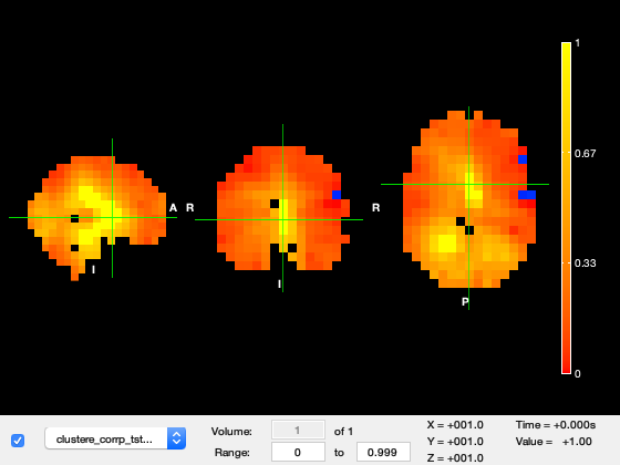
This opens up fslview showing the results. Take a look. The images include:

As with the previous cell - once you have run this section, try re-running to look at the window between 90 and 120 ms after stimulus onset. What differences do you notice between the early (90-120ms) and later (140-150ms) responses?

S=[];
S.oat=oat;
S.cluster_stats_thresh=6;
S.cluster_stats_nperms=1000; % we normally recommend doing 5000 perms
S.first_level_copes_to_do=[3];
S.group_level_copes_to_do=[1];
S.group_varcope_spatial_smooth_fwhm=S.oat.group_level.group_varcope_spatial_smooth_fwhm;
S.write_cluster_script=0;
S.time_range=[0.140 0.150];
S.time_average=1;

% Run the permutations
[ gstats ] = oat_cluster_permutation_testing( S );

% View permutation stats
con=S.first_level_copes_to_do(1);

tstat = fullfile(gstats.dir,['tstat' num2str(con) '_gc1_' num2str(gstats.gridstep) 'mm.nii.gz']);
clus_tstat = fullfile(gstats.dir,['clustere_tstat' num2str(con) '_gc1_' num2str(gstats.gridstep) 'mm.nii.gz']);
corr_clus_tstat = fullfile(gstats.dir,['clustere_corrp_tstat' num2str(con) '_gc1_' num2str(gstats.gridstep) 'mm.nii.gz']);

osleyes( {[],tstat, clus_tstat, corr_clus_tstat} );

Doing cluster perm testing
Warning: Directory already exists. 
Using max of mask over time window
Cluster 4D perm testing on group contrast 1
Warning: Directory already exists. 
randomise -d /Users/andrew/toolboxes/osl/example_data/faces_group_data/beamform.oat/first_level_none_sub_level_time_average_group_level_randomise_c3_dir/design.mat -t /Users/andrew/toolboxes/osl/example_data/faces_group_data/beamform.oat/first_level_none_sub_level_time_average_group_level_randomise_c3_dir/design.con -i /Users/andrew/toolboxes/osl/example_data/faces_group_data/beamform.oat/first_level_none_sub_level_time_average_group_level_randomise_c3_dir/allsubs_time0001 -o /Users/andrew/toolboxes/osl/example_data/faces_group_data/beamform.oat/first_level_none_sub_level_time_average_group_level_randomise_c3_dir/stats -c 6 -R -n 1000 --seed=0 -v 43.4783 -m /Users/andrew/toolboxes/osl/example_data/faces_group_data/beamform.oat/first_level_none_sub_level_time_average_group_level_randomise_c3_dir/mask_time0001

ROI TIME-FREQ ANALYSIS

We will now run an ROI power analysis over multiple frequency bands The oat.group_level.space_average=1 indicates that we want to do spatial averaging over the ROI at the group level (the averaging occurs before the group GLM is fit).

We first load in an OAT where the first three stages have been run for you, and here we will just run the group analysis. The OAT is being carried out (from the beamforming, source reconstruction, onwards) within a mask.

Type oat.source_recon.mask_fname to see which mask is being used.

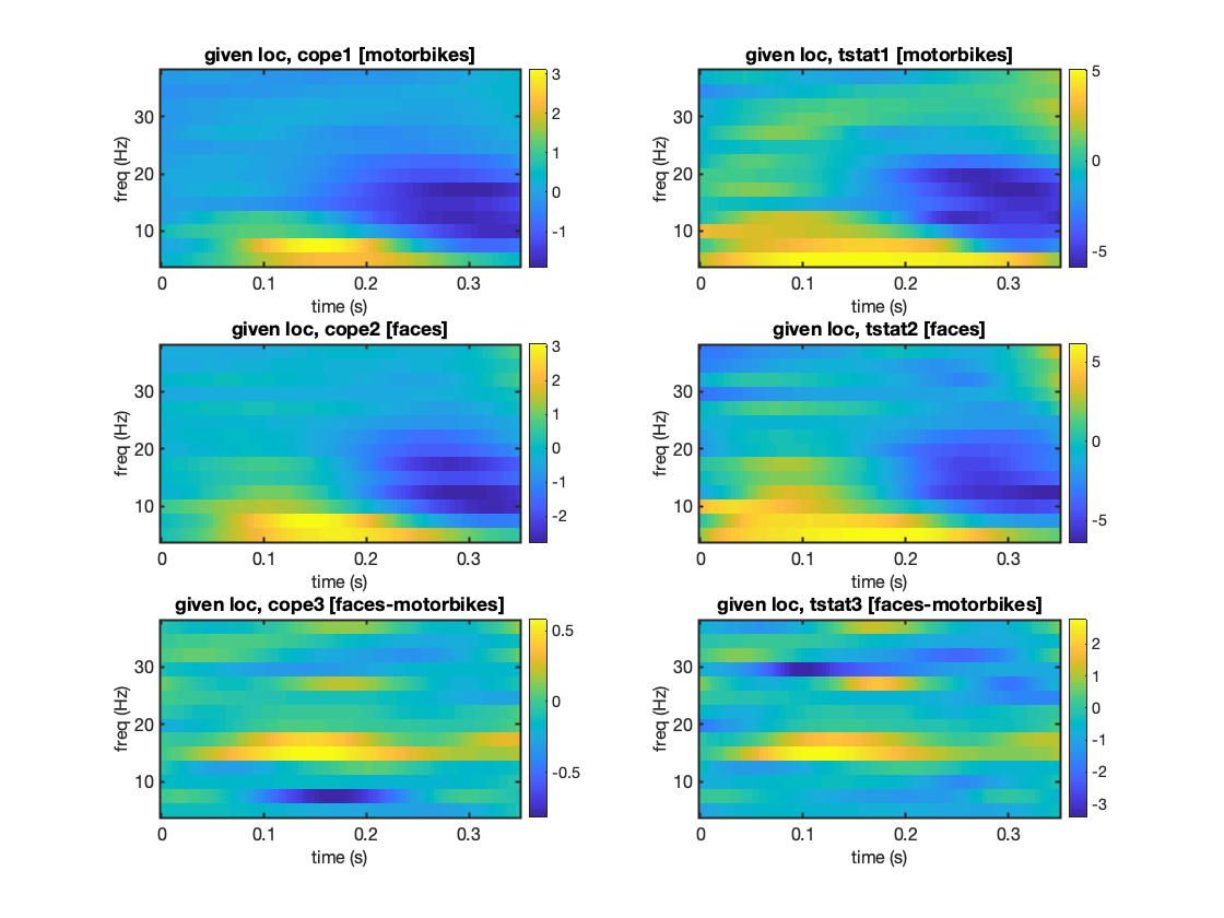
Next we run the group stage of OAT. This will bring up an image showing the time-frequency COPEs and t-statistics for the different contrasts.

% load in an OAT for which the first 3 stages have been run to do an ROI
% analysis using the Right_Temporal_Occipital_Fusiform mask
oat = osl_load_oat(fullfile(osldir,'example_data','faces_group_data','beamform_roi'), 'first_level_hilbert','sub_level','group_level');

% setup Group level of OAT and run
oat.group_level.time_range=oat.first_level.time_range;
oat.group_level.space_average=1;
oat.group_level.time_average=0;
oat.group_level.time_smooth_std=0; % secs
oat.group_level.spatial_smooth_fwhm=0; % mm
oat.group_level.use_tstat=1;
oat.group_level.name='group_level';
oat.group_level.store_lower_level_copes=1;
oat.group_level.subjects_to_do=[3:14];
oat.group_level.time_range=[0 0.35];

% Check and run the group level
oat=osl_check_oat(oat);
oat.to_do=[0 0 0 1];
oat=osl_run_oat(oat);

% Save the group results spatially averaged over an ROI
S2=[];
S2.oat=oat;
S2.stats_fname=oat.group_level.results_fnames;
S2.mask_fname=fullfile(osldir,'example_data','faces_group_data','structurals','Right_Temporal_Occipital_Fusiform_Cortex_8mm.nii.gz');
[stats,times,mni_coords_used]=oat_output_roi_stats(S2);

% Plot the Time-Frequency results
S2=[];
S2.stats=stats;
S2.oat=oat;
[vox_ind_used] = oat_plot_vox_stats(S2);

Loaded OAT: /Users/andrew/toolboxes/osl/example_data/faces_group_data/beamform_roi.oat/oat_first_level_hilbert_sub_level_group_level.mat
Unknown datatype. Using default Elekta Neuromag 306 settings
Warning: oat.source_recon.modalities not set, or not set properly. Will set to
default:MEGPLANARMEGMAG 
oat.source_recon.D_epoched set. OAT will do an epoched data trial-wise GLM
Unknown datatype. Using default Elekta Neuromag 306 settings
Warning: oat.source_recon.modalities not set, or not set properly. Will set to
default:MEGPLANARMEGMAG 
oat.source_recon.D_epoched set. OAT will do an epoched data trial-wise GLM
*************************************************************
Running group_level
*************************************************************
Loading in lower level stats
Using same indices as lower_level
 - estimated time to finish is 0 seconds
Processing Group stats for first level contrast 1, motorbikes
Number 1 of 3
Preparing data
Computing group statistics
 - estimated time to finish is NaN seconds
Processing Group stats for first level contrast 2, faces
Number 2 of 3
Preparing data
Computing group statistics
 - estimated time to finish is NaN seconds
Processing Group stats for first level contrast 3, faces-motorbikes
Number 3 of 3
Preparing data
Computing group statistics
 - estimated time to finish is NaN seconds
Processing Group stats for first level contrast 3 [faces-motorbikes]
Number 1 of 3
To view group level report, point your browser to <a href="/Users/andrew/toolboxes/osl/example_data/faces_group_data/beamform_roi.oat/plots/first_level_hilbert_sub_level_group_level/report.html">/Users/andrew/toolboxes/osl/example_data/faces_group_data/beamform_roi.oat/plots/first_level_hilbert_sub_level_group_level/report.html</a>
Saving statistics in file /Users/andrew/toolboxes/osl/example_data/faces_group_data/beamform_roi.oat/first_level_hilbert_sub_level_group_level
To view group level report, point your browser to <a href="/Users/andrew/toolboxes/osl/example_data/faces_group_data/beamform_roi.oat/plots/first_level_hilbert_sub_level_group_level/report.html">/Users/andrew/toolboxes/osl/example_data/faces_group_data/beamform_roi.oat/plots/first_level_hilbert_sub_level_group_level/report.html</a>
To view OAT report, point your browser to <a href="/Users/andrew/toolboxes/osl/example_data/faces_group_data/beamform_roi.oat/plots/report.html">/Users/andrew/toolboxes/osl/example_data/faces_group_data/beamform_roi.oat/plots/report.html</a>

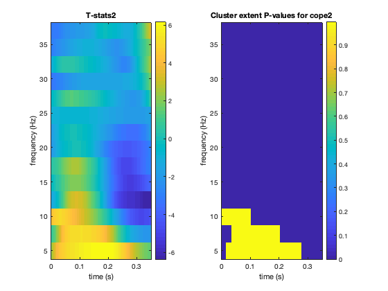
2D CLUSTER PERMUTATION STATS

Perform sign-flip permutation tests on the data from a single point in the time-frequency OAT. This is done on first level contrast 2 (face grand mean). This tells us which points in the time frequency analysis are statistically significant with p-values corrected for multiple comparisons and cluster size.

% load GLM result
stats=oat_load_results(oat,oat.group_level.results_fnames);

contrast=2; % first level contrast
cluster_forming_threshold=3.5; % threshold used on t-stats to form clusters
num_perms=1000; % num permutations to do - normally recommend doing 5000

% call osl_clustertf to do permutation testing
% this returns corrp, the corrected (over multiple comparisons) P-Value for
% each cluster in a 2D time-freq map
[corrp tstats]= osl_clustertf(permute(stats.lower_level_copes{contrast},[2 4 3 1]),cluster_forming_threshold,num_perms,26);

figure;
subplot(1,2,1);imagesc(stats.times, stats.frequencies, squeeze(tstats));axis xy;
ylabel('frequency (Hz)'); xlabel('time (s)'); colorbar; title(['T-stats' num2str(contrast)]);
subplot(1,2,2);imagesc(stats.times, stats.frequencies, squeeze(corrp));axis xy;
ylabel('frequency (Hz)'); xlabel('time (s)'); colorbar; title(['Cluster extent P-values for cope' num2str(contrast)]);

Published with MATLAB® R2019a